Note
Click here to download the full example code
A from scratch example on the Sellar problem
Introduction
In this example,
we will create an MDO scenario based on the Sellar’s problem from scratch.
Contrary to the GEMSEO in ten minutes tutorial,
all the disciplines will be implemented from scratch
by sub-classing the MDODiscipline class
for each discipline of the Sellar problem.
The Sellar problem
We will consider in this example the Sellar problem:
where the coupling variables are
and
and where the general constraints are
Imports
All the imports needed for the tutorials are performed here.
from __future__ import annotations

from math import exp

from gemseo.algos.design_space import DesignSpace
from gemseo.api import configure_logger
from gemseo.api import create_scenario
from gemseo.core.discipline import MDODiscipline
from matplotlib import pyplot as plt
from numpy import array
from numpy import ones

configure_logger()
<RootLogger root (INFO)>
Create the disciplinary classes
In this section,
we define the Sellar disciplines by sub-classing the MDODiscipline class.
For each class,
the constructor and the _run method are overriden:
In the constructor, the input and output grammar are created. They define which inputs and outputs variables are allowed at the discipline execution. The default inputs are also defined, in case of the user does not provide them at the discipline execution.
In the _run method is implemented the concrete computation of the discipline. The inputs data are fetch by using the
MDODiscipline.get_inputs_by_name()method. The returned NumPy arrays can then be used to compute the output values. They can then be stored in theMDODiscipline.local_datadictionary. If the discipline execution is successful.
Note that we do not define the Jacobians in the disciplines. In this example, we will approximate the derivatives using the finite differences method.
Create the SellarSystem class
class SellarSystem(MDODiscipline):
    def __init__(self):
        super().__init__()
        # Initialize the grammars to define inputs and outputs
        self.input_grammar.update(["x", "z", "y_1", "y_2"])
        self.output_grammar.update(["obj", "c_1", "c_2"])
        # Default inputs define what data to use when the inputs are not
        # provided to the execute method
        self.default_inputs = {
            "x": ones(1),
            "z": array([4.0, 3.0]),
            "y_1": ones(1),
            "y_2": ones(1),
        }

    def _run(self):
        # The run method defines what happens at execution
        # ie how outputs are computed from inputs
        x, z, y_1, y_2 = self.get_inputs_by_name(["x", "z", "y_1", "y_2"])
        # The ouputs are stored here
        self.local_data["obj"] = array([x[0] ** 2 + z[1] + y_1[0] ** 2 + exp(-y_2[0])])
        self.local_data["c_1"] = array([3.16 - y_1[0] ** 2])
        self.local_data["c_2"] = array([y_2[0] - 24.0])
Create the Sellar1 class
class Sellar1(MDODiscipline):
    def __init__(self):
        super().__init__()
        self.input_grammar.update(["x", "z", "y_2"])
        self.output_grammar.update(["y_1"])
        self.default_inputs = {
            "x": ones(1),
            "z": array([4.0, 3.0]),
            "y_1": ones(1),
            "y_2": ones(1),
        }

    def _run(self):
        x, z, y_2 = self.get_inputs_by_name(["x", "z", "y_2"])
        self.local_data["y_1"] = array(
            [(z[0] ** 2 + z[1] + x[0] - 0.2 * y_2[0]) ** 0.5]
        )
Create the Sellar2 class
class Sellar2(MDODiscipline):
    def __init__(self):
        super().__init__()
        self.input_grammar.update(["z", "y_1"])
        self.output_grammar.update(["y_2"])
        self.default_inputs = {
            "x": ones(1),
            "z": array([4.0, 3.0]),
            "y_1": ones(1),
            "y_2": ones(1),
        }

    def _run(self):
        z, y_1 = self.get_inputs_by_name(["z", "y_1"])
        self.local_data["y_2"] = array([abs(y_1[0]) + z[0] + z[1]])
Create and execute the scenario
Instantiate disciplines
We can now instantiate the disciplines and store the instances in a list which will be used below.
disciplines = [Sellar1(), Sellar2(), SellarSystem()]
Create the design space
In this section, we define the design space which will be used for the creation of the MDOScenario. Note that the coupling variables are defined in the design space. Indeed, as we are going to select the IDF formulation to solve the MDO scenario, the coupling variables will be unknowns of the optimization problem and consequently they have to be included in the design space. Conversely, it would not have been necessary to include them if we aimed to select an MDF formulation.
design_space = DesignSpace()
design_space.add_variable("x", 1, l_b=0.0, u_b=10.0, value=ones(1))
design_space.add_variable(
    "z", 2, l_b=(-10, 0.0), u_b=(10.0, 10.0), value=array([4.0, 3.0])
)
design_space.add_variable("y_1", 1, l_b=-100.0, u_b=100.0, value=ones(1))
design_space.add_variable("y_2", 1, l_b=-100.0, u_b=100.0, value=ones(1))
Create the scenario
In this section, we build the MDO scenario which links the disciplines with the formulation, the design space and the objective function.
scenario = create_scenario(
    disciplines, formulation="IDF", objective_name="obj", design_space=design_space
)
Add the constraints
Then, we have to set the design constraints
scenario.add_constraint("c_1", "ineq")
scenario.add_constraint("c_2", "ineq")
As previously mentioned, we are going to use finite differences to approximate the derivatives since the disciplines do not provide them.
scenario.set_differentiation_method("finite_differences", 1e-6)
Execute the scenario
Then, we execute the MDO scenario with the inputs of the MDO scenario as a dictionary. In this example, the gradient-based SLSQP optimizer is selected, with 10 iterations at maximum:
scenario.execute(input_data={"max_iter": 10, "algo": "SLSQP"})
    INFO - 14:47:16:
    INFO - 14:47:16: *** Start MDOScenario execution ***
    INFO - 14:47:16: MDOScenario
    INFO - 14:47:16:    Disciplines: Sellar1 Sellar2 SellarSystem
    INFO - 14:47:16:    MDO formulation: IDF
    INFO - 14:47:16: Optimization problem:
    INFO - 14:47:16:    minimize obj(x, z, y_1, y_2)
    INFO - 14:47:16:    with respect to x, y_1, y_2, z
    INFO - 14:47:16:    subject to constraints:
    INFO - 14:47:16:       c_1(x, z, y_1, y_2) <= 0.0
    INFO - 14:47:16:       c_2(x, z, y_1, y_2) <= 0.0
    INFO - 14:47:16:       y_1: y_1(x, z, y_2): y_1(x, z, y_2) - y_1 == 0.0
    INFO - 14:47:16:       y_2: y_2(z, y_1): y_2(z, y_1) - y_2 == 0.0
    INFO - 14:47:16:    over the design space:
    INFO - 14:47:16:    +------+-------------+-------+-------------+-------+
    INFO - 14:47:16:    | name | lower_bound | value | upper_bound | type  |
    INFO - 14:47:16:    +------+-------------+-------+-------------+-------+
    INFO - 14:47:16:    | x    |      0      |   1   |      10     | float |
    INFO - 14:47:16:    | z[0] |     -10     |   4   |      10     | float |
    INFO - 14:47:16:    | z[1] |      0      |   3   |      10     | float |
    INFO - 14:47:16:    | y_1  |     -100    |   1   |     100     | float |
    INFO - 14:47:16:    | y_2  |     -100    |   1   |     100     | float |
    INFO - 14:47:16:    +------+-------------+-------+-------------+-------+
    INFO - 14:47:16: Solving optimization problem with algorithm SLSQP:
    INFO - 14:47:16: ...   0%|          | 0/10 [00:00<?, ?it]
    INFO - 14:47:16: ...  60%|██████    | 6/10 [00:00<00:00, 119.48 it/sec, obj=3.18]
    INFO - 14:47:16: Optimization result:
    INFO - 14:47:16:    Optimizer info:
    INFO - 14:47:16:       Status: 8
    INFO - 14:47:16:       Message: Positive directional derivative for linesearch
    INFO - 14:47:16:       Number of calls to the objective function by the optimizer: 7
    INFO - 14:47:16:    Solution:
    INFO - 14:47:16:       The solution is feasible.
    INFO - 14:47:16:       Objective: 3.1833939516400456
    INFO - 14:47:16:       Standardized constraints:
    INFO - 14:47:16:          c_1 = 5.764277943853813e-13
    INFO - 14:47:16:          c_2 = -20.244722233074114
    INFO - 14:47:16:          y_1 = [2.06834549e-15]
    INFO - 14:47:16:          y_2 = [1.98063788e-15]
    INFO - 14:47:16:       Design space:
    INFO - 14:47:16:       +------+-------------+-------------------+-------------+-------+
    INFO - 14:47:16:       | name | lower_bound |       value       | upper_bound | type  |
    INFO - 14:47:16:       +------+-------------+-------------------+-------------+-------+
    INFO - 14:47:16:       | x    |      0      |         0         |      10     | float |
    INFO - 14:47:16:       | z[0] |     -10     | 1.977638883463326 |      10     | float |
    INFO - 14:47:16:       | z[1] |      0      |         0         |      10     | float |
    INFO - 14:47:16:       | y_1  |     -100    | 1.777638883462956 |     100     | float |
    INFO - 14:47:16:       | y_2  |     -100    | 3.755277766925886 |     100     | float |
    INFO - 14:47:16:       +------+-------------+-------------------+-------------+-------+
    INFO - 14:47:16: *** End MDOScenario execution (time: 0:00:00.097537) ***

{'max_iter': 10, 'algo': 'SLSQP'}
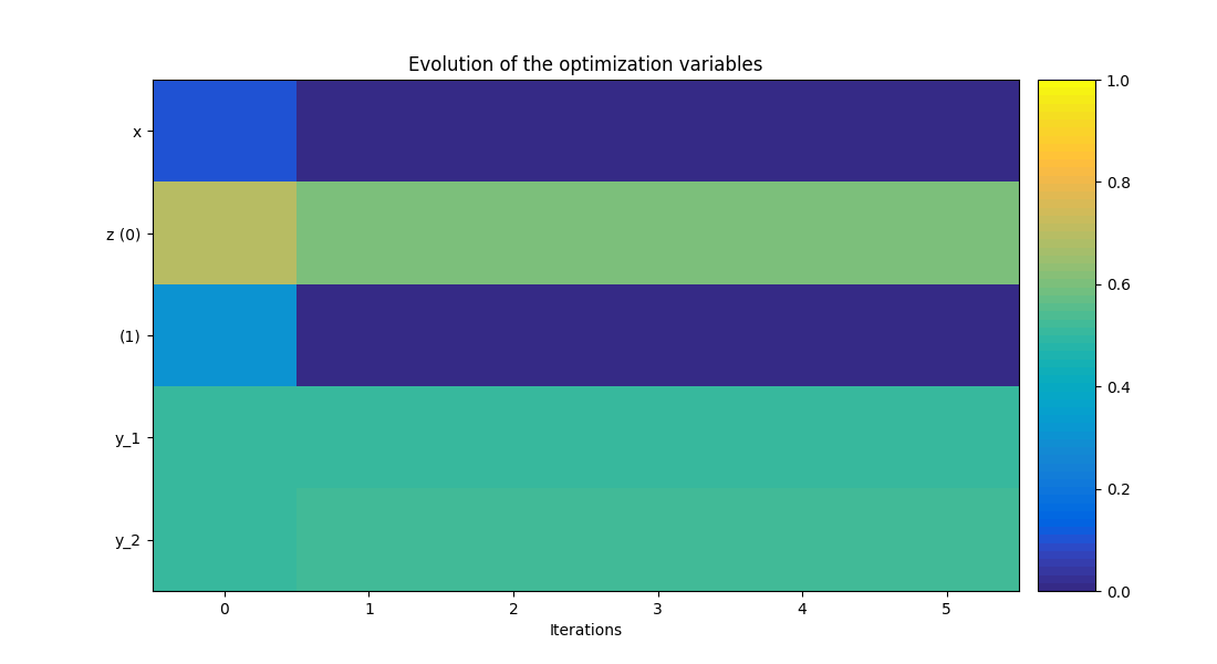
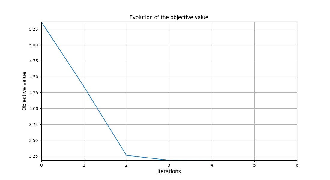
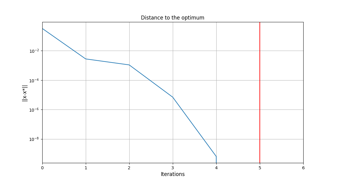
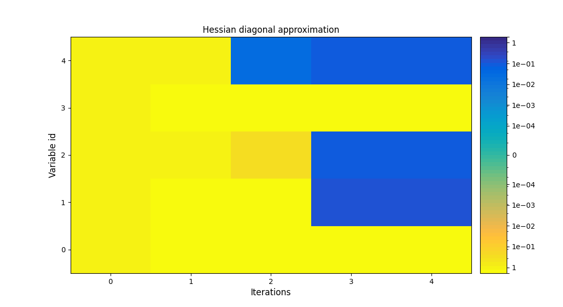
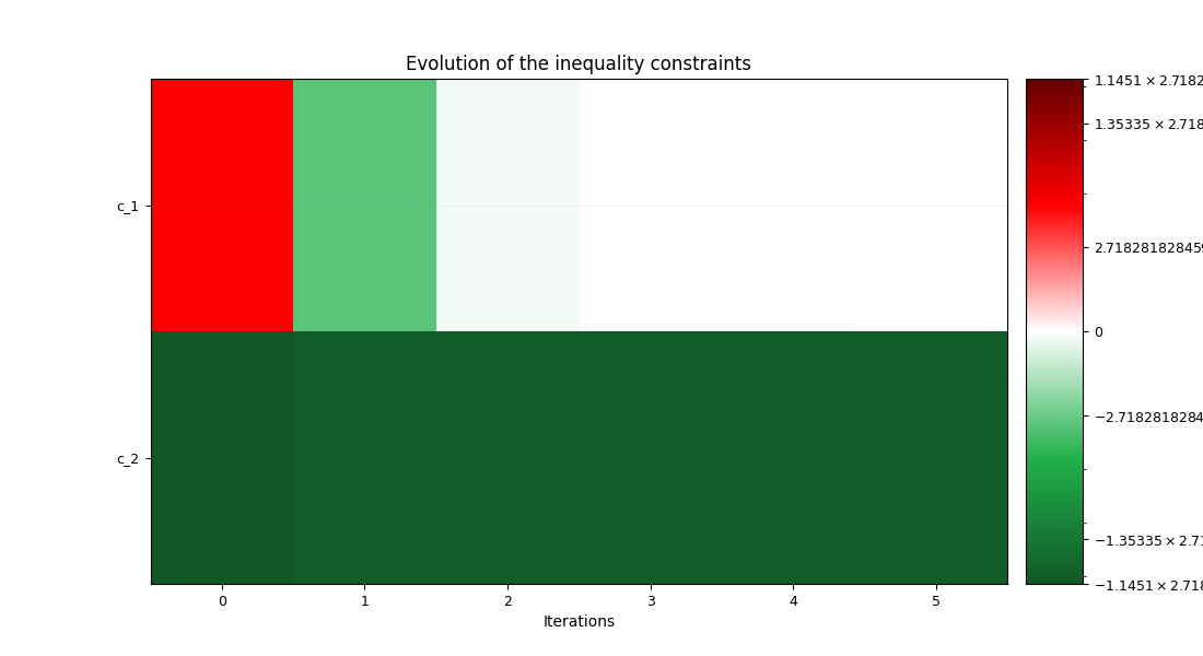
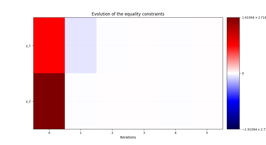
Post-process the scenario
Finally, we can generate plots of the optimization history:
scenario.post_process("OptHistoryView", save=False, show=False)
# Workaround for HTML rendering, instead of ``show=True``
plt.show()
Total running time of the script: ( 0 minutes 1.389 seconds)