Note
Click here to download the full example code
GEMSEO in 10 minutes
Introduction
This is a short introduction to GEMSEO, geared mainly for new users. In this example, we will set up a simple Multi-disciplinary Design Optimization (MDO) problem based on a simple analytic problem.
Imports
First, we will import all the classes and functions needed for the tutorials.
from __future__ import annotations

from math import exp

from gemseo.api import configure_logger
from gemseo.api import create_design_space
from gemseo.api import create_discipline
from gemseo.api import create_scenario
from gemseo.api import generate_n2_plot
from matplotlib import pyplot as plt
from numpy import array
from numpy import ones
These imports are needed to compute mathematical expressions and to instantiate NumPy arrays. NumPy arrays are used to store numerical data in GEMSEO at a low level. If you are not comfortable using NumPy, please have a look at the Numpy Quickstart tutorial.
Here, we configure the GEMSEO logger in order to get information of the process as it is executed.
configure_logger()
<RootLogger root (INFO)>
A simple MDO test case: the Sellar Problem
We will consider in this example the Sellar’s problem:
where the coupling variables are
and
and where the general constraints are
Definition of the disciplines using Python functions
The Sellar’s problem is composed of two disciplines and an objective function. As they are expressed analytically, it is possible to write them as simple Python functions which take as parameters the design variables and the coupling variables. The returned values may be the outputs of a discipline, the values of the constraints or the value of the objective function. Their definitions read:
def f_sellar_system(x_local=1.0, x_shared_2=3.0, y_1=1.0, y_2=1.0):
    """Objective function."""
    obj = x_local**2 + x_shared_2 + y_1**2 + exp(-y_2)
    c_1 = 3.16 - y_1**2
    c_2 = y_2 - 24.0
    return obj, c_1, c_2


def f_sellar_1(x_local=1.0, y_2=1.0, x_shared_1=1.0, x_shared_2=3.0):
    """Function for discipline 1."""
    y_1 = (x_shared_1**2 + x_shared_2 + x_local - 0.2 * y_2) ** 0.5
    return y_1


def f_sellar_2(y_1=1.0, x_shared_1=1.0, x_shared_2=3.0):
    """Function for discipline 2."""
    y_2 = abs(y_1) + x_shared_1 + x_shared_2
    return y_2
These Python functions can be easily converted into GEMSEO
MDODiscipline objects by using the AutoPyDiscipline
discipline. It enables the automatic wrapping of a Python function into a
GEMSEO
MDODiscipline by only passing a reference to the function to be
wrapped. GEMSEO handles the wrapping and the grammar creation under the
hood. The AutoPyDiscipline discipline can be instantiated using the
create_discipline() function from the GEMSEO API:
disc_sellar_system = create_discipline("AutoPyDiscipline", py_func=f_sellar_system)

disc_sellar_1 = create_discipline("AutoPyDiscipline", py_func=f_sellar_1)

disc_sellar_2 = create_discipline("AutoPyDiscipline", py_func=f_sellar_2)
Note that it is possible to define the Sellar disciplines by subclassing the
MDODiscipline class and implementing the constuctor and the _run
method by hand. Although it would take more time, it may also provide more
flexibility and more options. This method is illustrated in the Sellar
from scratch tutorial.
We then create a list of disciplines, which will be used later to create an
MDOScenario:
disciplines = [disc_sellar_system, disc_sellar_1, disc_sellar_2]
We can quickly access the most relevant information of any discipline (name, inputs,
and outputs) with Python’s print() function. Moreover, we can get the default
input values of a discipline with the attribute MDODiscipline.default_inputs
print(disc_sellar_1)
print(f"Default inputs: {disc_sellar_1.default_inputs}")
f_sellar_1
Default inputs: {'x_local': array([1.]), 'y_2': array([1.]), 'x_shared_1': array([1.]), 'x_shared_2': array([3.])}
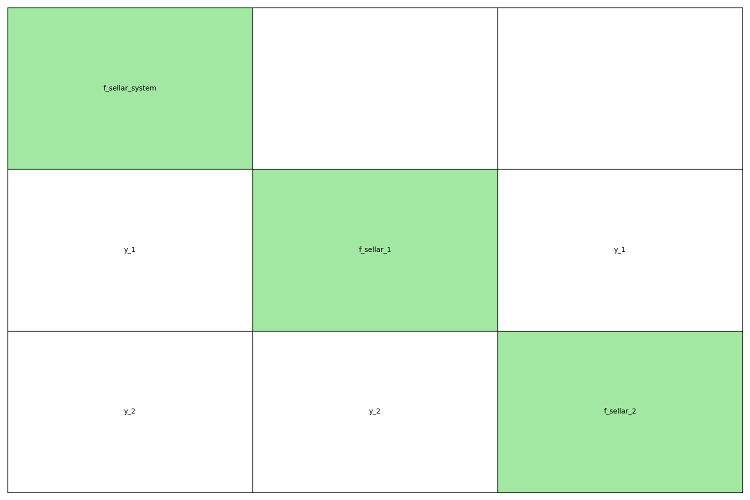
You may also be interested in plotting the couplings of your disciplines.
A quick way of getting this information is the API function
generate_n2_plot(). A much more detailed explanation of coupling
visualization is available here.
generate_n2_plot(disciplines, save=False, show=True)
Note
For the sake of clarity, these disciplines are overly simple. Yet, GEMSEO enables the definition of much more complex disciplines, such as wrapping complex COTS. Check out the other tutorials and our publications list for more information.
Definition of the design space
In order to define MDOScenario,
a design space has to be defined by creating a DesignSpace
object. The design space definition reads:
design_space = create_design_space()
design_space.add_variable("x_local", 1, l_b=0.0, u_b=10.0, value=ones(1))
design_space.add_variable("x_shared_1", 1, l_b=-10, u_b=10.0, value=array([4.0]))
design_space.add_variable("x_shared_2", 1, l_b=0.0, u_b=10.0, value=array([3.0]))
design_space.add_variable("y_1", 1, l_b=-100.0, u_b=100.0, value=ones(1))
design_space.add_variable("y_2", 1, l_b=-100.0, u_b=100.0, value=ones(1))
print(design_space)
Design space:
+------------+-------------+-------+-------------+-------+
| name       | lower_bound | value | upper_bound | type  |
+------------+-------------+-------+-------------+-------+
| x_local    |      0      |   1   |      10     | float |
| x_shared_1 |     -10     |   4   |      10     | float |
| x_shared_2 |      0      |   3   |      10     | float |
| y_1        |     -100    |   1   |     100     | float |
| y_2        |     -100    |   1   |     100     | float |
+------------+-------------+-------+-------------+-------+
Definition of the MDO scenario
Once the disciplines and the design space have been defined,
we can create our MDO scenario by using the create_scenario()
API call. In this simple example,
we are using a Multiple Disciplinary Feasible (MDF) strategy.
The Multiple Disciplinary Analyses (MDA) are carried out using the
Gauss-Seidel method. The scenario definition reads:
scenario = create_scenario(
    disciplines,
    formulation="MDF",
    inner_mda_name="MDAGaussSeidel",
    objective_name="obj",
    design_space=design_space,
)
It can be noted that neither a workflow nor a dataflow has been defined. By design, there is no need to explicitly define the workflow and the dataflow in GEMSEO:
the workflow is determined from the MDO formulation used.
the dataflow is determined from the variable names used in the disciplines. Then, it is of uttermost importance to be consistent while choosing and using the variable names in the disciplines.
Warning
As the workflow and the dataflow are implicitly determined by GEMSEO, set-up errors may easily occur. Although it is not performed in this example, it is strongly advised to
check the interfaces between the several disciplines using an N2 diagram,
check the MDO process using an XDSM representation
Setting the constraints
Most of the MDO problems are under constraints. In our problem, we have two inequality constraints, and their declaration reads:
scenario.add_constraint("c_1", "ineq")
scenario.add_constraint("c_2", "ineq")
Execution of the scenario
The scenario is now complete and ready to be executed. When running the optimization process, the user can choose the optimization algorithm and the maximum number of iterations to perform. The execution of the scenario reads:
scenario.execute(input_data={"max_iter": 10, "algo": "SLSQP"})
    INFO - 14:47:23:
    INFO - 14:47:23: *** Start MDOScenario execution ***
    INFO - 14:47:23: MDOScenario
    INFO - 14:47:23:    Disciplines: f_sellar_1 f_sellar_2 f_sellar_system
    INFO - 14:47:23:    MDO formulation: MDF
    INFO - 14:47:23: Optimization problem:
    INFO - 14:47:23:    minimize obj(x_local, x_shared_1, x_shared_2)
    INFO - 14:47:23:    with respect to x_local, x_shared_1, x_shared_2
    INFO - 14:47:23:    subject to constraints:
    INFO - 14:47:23:       c_1(x_local, x_shared_1, x_shared_2) <= 0.0
    INFO - 14:47:23:       c_2(x_local, x_shared_1, x_shared_2) <= 0.0
    INFO - 14:47:23:    over the design space:
    INFO - 14:47:23:    +------------+-------------+-------+-------------+-------+
    INFO - 14:47:23:    | name       | lower_bound | value | upper_bound | type  |
    INFO - 14:47:23:    +------------+-------------+-------+-------------+-------+
    INFO - 14:47:23:    | x_local    |      0      |   1   |      10     | float |
    INFO - 14:47:23:    | x_shared_1 |     -10     |   4   |      10     | float |
    INFO - 14:47:23:    | x_shared_2 |      0      |   3   |      10     | float |
    INFO - 14:47:23:    +------------+-------------+-------+-------------+-------+
    INFO - 14:47:23: Solving optimization problem with algorithm SLSQP:
    INFO - 14:47:23: ...   0%|          | 0/10 [00:00<?, ?it]
    INFO - 14:47:23: ...  30%|███       | 3/10 [00:00<00:00, 90.30 it/sec, obj=3.41]
    INFO - 14:47:23: ...  60%|██████    | 6/10 [00:00<00:00, 44.91 it/sec, obj=3.18]
    INFO - 14:47:23: ...  80%|████████  | 8/10 [00:00<00:00, 33.62 it/sec, obj=3.18]
    INFO - 14:47:23: Optimization result:
    INFO - 14:47:23:    Optimizer info:
    INFO - 14:47:23:       Status: None
    INFO - 14:47:23:       Message: Successive iterates of the objective function are closer than ftol_rel or ftol_abs. GEMSEO Stopped the driver
    INFO - 14:47:23:       Number of calls to the objective function by the optimizer: 9
    INFO - 14:47:23:    Solution:
    INFO - 14:47:23:       The solution is feasible.
    INFO - 14:47:23:       Objective: 3.1833939496730377
    INFO - 14:47:23:       Standardized constraints:
    INFO - 14:47:23:          c_1 = 2.5499602429590595e-12
    INFO - 14:47:23:          c_2 = -20.24472214907656
    INFO - 14:47:23:       Design space:
    INFO - 14:47:23:       +------------+-------------+------------------+-------------+-------+
    INFO - 14:47:23:       | name       | lower_bound |      value       | upper_bound | type  |
    INFO - 14:47:23:       +------------+-------------+------------------+-------------+-------+
    INFO - 14:47:23:       | x_local    |      0      |        0         |      10     | float |
    INFO - 14:47:23:       | x_shared_1 |     -10     | 1.97763896746104 |      10     | float |
    INFO - 14:47:23:       | x_shared_2 |      0      |        0         |      10     | float |
    INFO - 14:47:23:       +------------+-------------+------------------+-------------+-------+
    INFO - 14:47:23: *** End MDOScenario execution (time: 0:00:00.309146) ***

{'max_iter': 10, 'algo': 'SLSQP'}
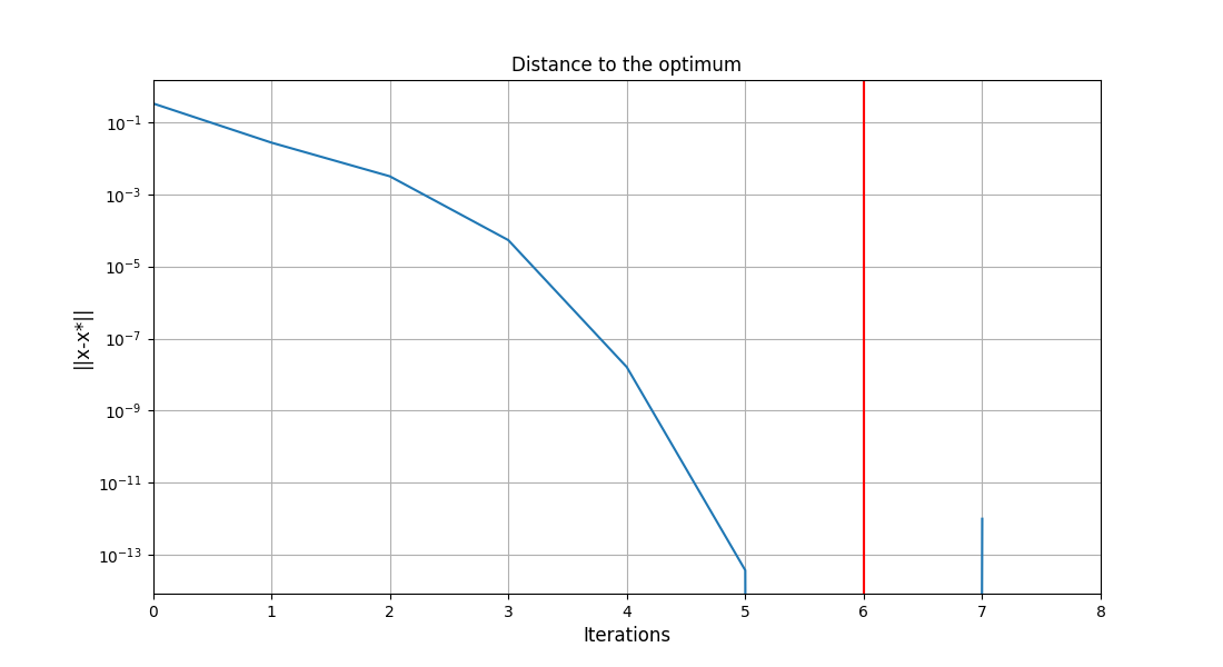
The scenario converged after 7 iterations. Useful information can be found in the standard output, as seen above.
Note
GEMSEO provides the user with a lot of optimization algorithms and options. An exhaustive list of the algorithms available in GEMSEO can be found in the Optimization algorithms section.
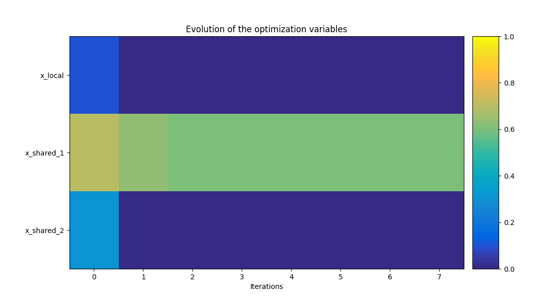
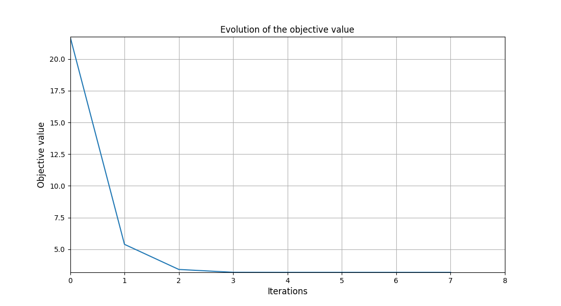
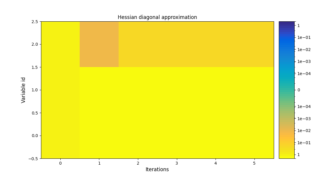
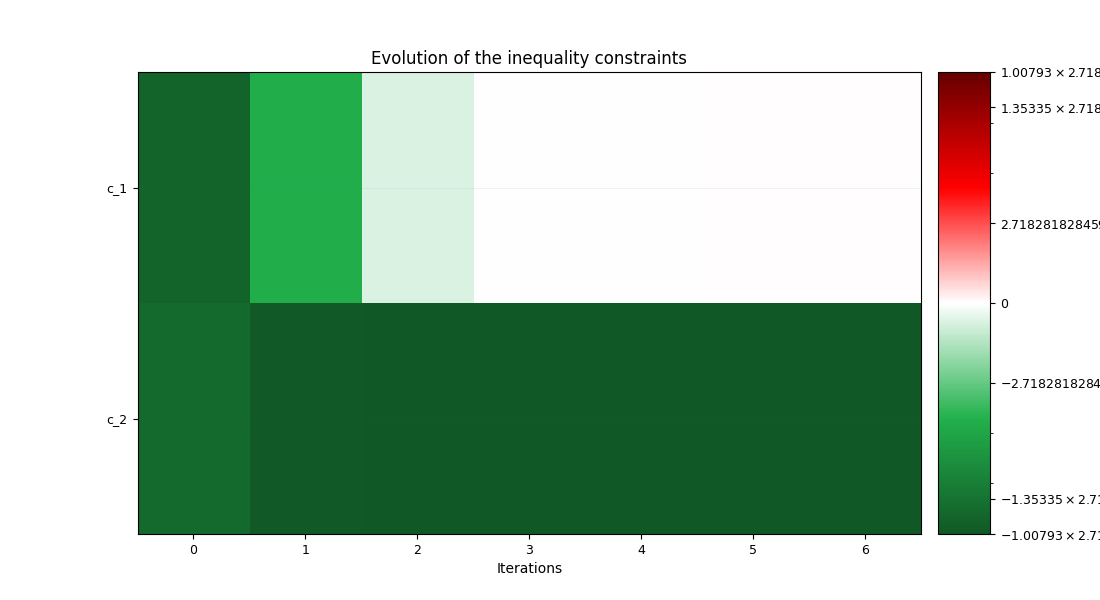
Post-processing the results
Post-processings such as plots exhibiting the evolutions of the objective function, the design variables or the constraints can be extremely useful. The convergence of the objective function, design variables and of the inequality constraints can be observed in the following plots. Many other post-processings are available in GEMSEO and are described in Post-processing.
scenario.post_process("OptHistoryView", save=False, show=False)
# Workaround for HTML rendering, instead of ``show=True``
plt.show()
Note
Such post-processings can be exported in PDF format,
by setting save to True and potentially additional
settings (see the Scenario.post_process() options).
Exporting the problem data.
After the execution of the scenario, you may want to export your data to use it
elsewhere. The Scenario.export_to_dataset() will allow you to export your
results to a Dataset, the basic GEMSEO class to store data.
From a dataset, you can even obtain a Pandas dataframe with its method
export_to_dataframe():
dataset = scenario.export_to_dataset("a_name_for_my_dataset")
dataframe = dataset.export_to_dataframe()
What’s next?
You have completed a short introduction to GEMSEO. You can now look at the tutorials which exhibit more complex use-cases. You can also have a look at the documentation to discover the several features and options of GEMSEO.
Total running time of the script: ( 0 minutes 1.681 seconds)