Scalable diagonal discipline

Let us consider the SobieskiAerodynamics discipline. We want to build its ScalableDiscipline counterpart, using a ScalableDiagonalModel

For that, we can use a 20-length DiagonalDOE and test different sizes of variables or different settings for the scalable diagonal discipline.

from __future__ import annotations

from gemseo.api import configure_logger
from gemseo.api import create_discipline
from gemseo.api import create_scalable
from gemseo.api import create_scenario
from gemseo.problems.sobieski.core.problem import SobieskiProblem
from matplotlib import pyplot as plt

Import

configure_logger()

<RootLogger root (INFO)>

Learning dataset

The first step is to build an AbstractFullCache dataset from a DiagonalDOE.

Instantiate the discipline

For that, we instantiate the SobieskiAerodynamics discipline and set it up to cache all evaluations.

discipline = create_discipline("SobieskiAerodynamics")

Get the input space

We also define the input space on which to sample the discipline.

input_space = SobieskiProblem().design_space
input_names = [name for name in discipline.get_input_data_names() if name != "c_4"]
input_space.filter(input_names)

<gemseo.algos.design_space.DesignSpace object at 0x7f3c13708ac0>

Build the DOE scenario

Lastly, we sample the discipline by means of a DOEScenario relying on both discipline and input space. In order to build a diagonal scalable discipline, a DiagonalDOE must be used.

scenario = create_scenario(
    [discipline], "DisciplinaryOpt", "y_2", input_space, scenario_type="DOE"
)
for output_name in discipline.get_output_data_names():
    if output_name != "y_2":
        scenario.add_observable(output_name)
scenario.execute({"algo": "DiagonalDOE", "n_samples": 20})

    INFO - 14:44:46:
    INFO - 14:44:46: *** Start DOEScenario execution ***
    INFO - 14:44:46: DOEScenario
    INFO - 14:44:46:    Disciplines: SobieskiAerodynamics
    INFO - 14:44:46:    MDO formulation: DisciplinaryOpt
    INFO - 14:44:46: Optimization problem:
    INFO - 14:44:46:    minimize y_2(x_shared, x_2, y_32, y_12)
    INFO - 14:44:46:    with respect to x_2, x_shared, y_12, y_32
    INFO - 14:44:46:    over the design space:
    INFO - 14:44:46:    +-------------+-------------+--------------------+-------------+-------+
    INFO - 14:44:46:    | name        | lower_bound |       value        | upper_bound | type  |
    INFO - 14:44:46:    +-------------+-------------+--------------------+-------------+-------+
    INFO - 14:44:46:    | x_shared[0] |     0.01    |        0.05        |     0.09    | float |
    INFO - 14:44:46:    | x_shared[1] |    30000    |       45000        |    60000    | float |
    INFO - 14:44:46:    | x_shared[2] |     1.4     |        1.6         |     1.8     | float |
    INFO - 14:44:46:    | x_shared[3] |     2.5     |        5.5         |     8.5     | float |
    INFO - 14:44:46:    | x_shared[4] |      40     |         55         |      70     | float |
    INFO - 14:44:46:    | x_shared[5] |     500     |        1000        |     1500    | float |
    INFO - 14:44:46:    | x_2         |     0.75    |         1          |     1.25    | float |
    INFO - 14:44:46:    | y_32        |    0.235    | 0.5027962499999999 |    0.795    | float |
    INFO - 14:44:46:    | y_12[0]     |    24850    |     50606.9742     |    77250    | float |
    INFO - 14:44:46:    | y_12[1]     |     0.45    |        0.95        |     1.5     | float |
    INFO - 14:44:46:    +-------------+-------------+--------------------+-------------+-------+
    INFO - 14:44:46: Solving optimization problem with algorithm DiagonalDOE:
    INFO - 14:44:46: ...   0%|          | 0/20 [00:00<?, ?it]
    INFO - 14:44:46: ... 100%|██████████| 20/20 [00:00<00:00, 451.45 it/sec, obj=[7.72500000e+04 1.27392070e+04 6.06395673e+00]]
    INFO - 14:44:46: Optimization result:
    INFO - 14:44:46:    Optimizer info:
    INFO - 14:44:46:       Status: None
    INFO - 14:44:46:       Message: None
    INFO - 14:44:46:       Number of calls to the objective function by the optimizer: 20
    INFO - 14:44:46:    Solution:
    INFO - 14:44:46:       Objective: 25508.372961119574
    INFO - 14:44:46:       Design space:
    INFO - 14:44:46:       +-------------+-------------+-------+-------------+-------+
    INFO - 14:44:46:       | name        | lower_bound | value | upper_bound | type  |
    INFO - 14:44:46:       +-------------+-------------+-------+-------------+-------+
    INFO - 14:44:46:       | x_shared[0] |     0.01    |  0.01 |     0.09    | float |
    INFO - 14:44:46:       | x_shared[1] |    30000    | 30000 |    60000    | float |
    INFO - 14:44:46:       | x_shared[2] |     1.4     |  1.4  |     1.8     | float |
    INFO - 14:44:46:       | x_shared[3] |     2.5     |  2.5  |     8.5     | float |
    INFO - 14:44:46:       | x_shared[4] |      40     |   40  |      70     | float |
    INFO - 14:44:46:       | x_shared[5] |     500     |  500  |     1500    | float |
    INFO - 14:44:46:       | x_2         |     0.75    |  0.75 |     1.25    | float |
    INFO - 14:44:46:       | y_32        |    0.235    | 0.235 |    0.795    | float |
    INFO - 14:44:46:       | y_12[0]     |    24850    | 24850 |    77250    | float |
    INFO - 14:44:46:       | y_12[1]     |     0.45    |  0.45 |     1.5     | float |
    INFO - 14:44:46:       +-------------+-------------+-------+-------------+-------+
    INFO - 14:44:46: *** End DOEScenario execution (time: 0:00:00.059042) ***

{'eval_jac': False, 'algo': 'DiagonalDOE', 'n_samples': 20}

Scalable diagonal discipline

Build the scalable discipline

The second step is to build a ScalableDiscipline, using a ScalableDiagonalModel and the database converted to a Dataset.

dataset = scenario.export_to_dataset(opt_naming=False)
scalable = create_scalable("ScalableDiagonalModel", dataset)

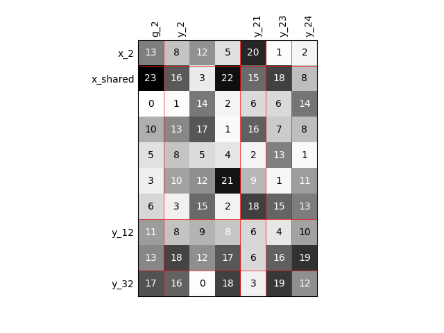
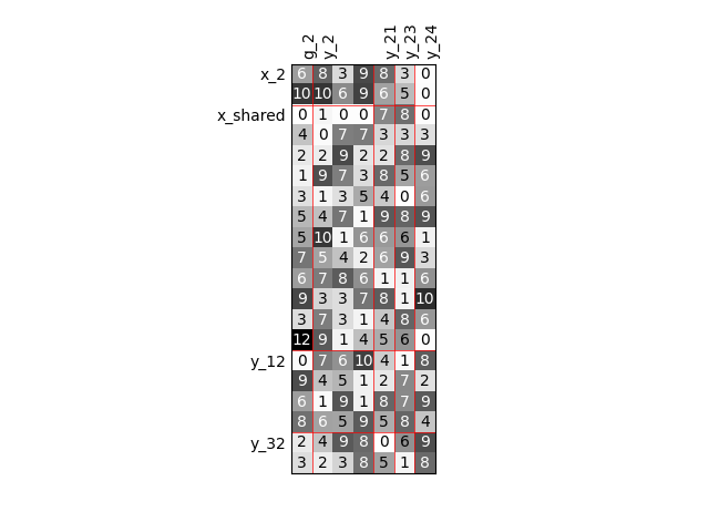
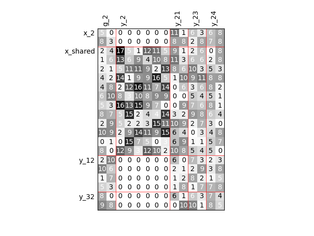
Visualize the input-output dependencies

We can easily access the underlying ScalableDiagonalModel and plot the corresponding input-output dependency matrix where the level of gray and the number (in [0,100]) represent the degree of dependency between inputs and outputs. Input are on the left while outputs are at the top. More precisely, for a given output component located at the top of the graph, these degrees are contributions to the output component and they add up to 1. In other words, a degree expresses this contribution in percentage and for a given column, the elements add up to 100.

scalable.scalable_model.plot_dependency(save=False, show=False)

'None'

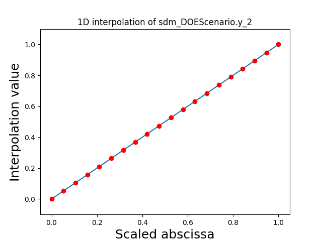
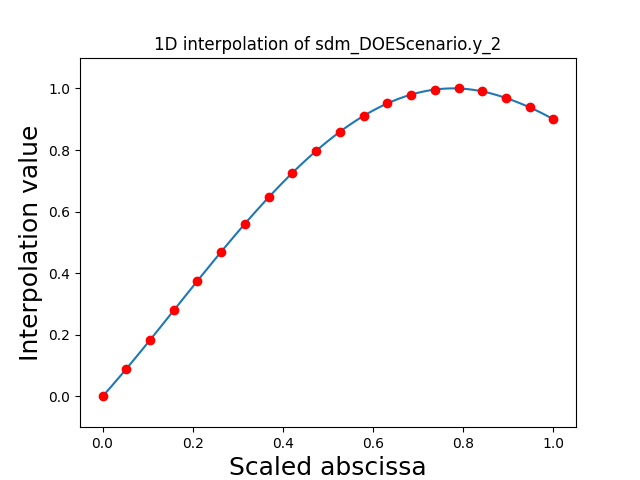
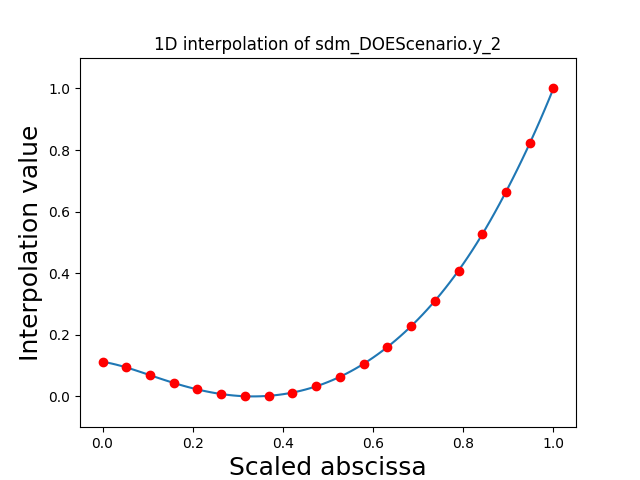
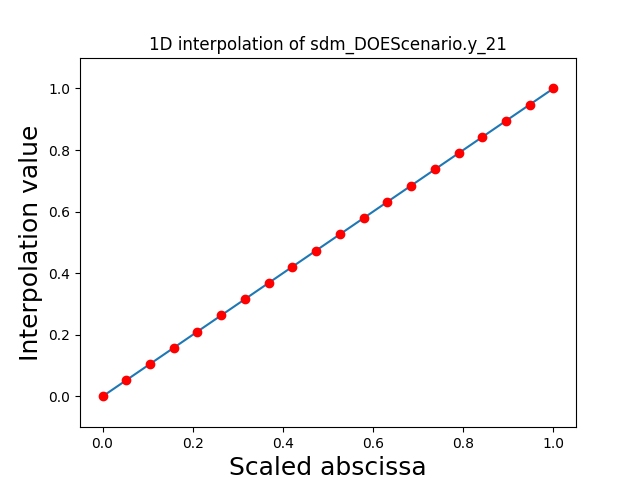
Visualize the 1D interpolations

For every output, we can also visualize a spline interpolation of the output samples over the diagonal of the input space.

scalable.scalable_model.plot_1d_interpolations(save=False, show=False)

• 
• 
• 
• 
• 
• 
• 

[]

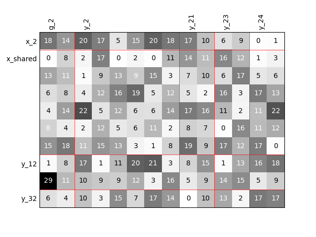
Increased problem dimension

We can repeat the construction of the scalable discipline for different sizes of variables and visualize the input-output dependency matrices.

Twice as many inputs

For example, we can increase the size of each input by a factor of 2.

sizes = {name: dataset.sizes[name] * 2 for name in input_names}
scalable = create_scalable("ScalableDiagonalModel", dataset, sizes)
scalable.scalable_model.plot_dependency(save=False, show=False)

'None'

Twice as many outputs

Or we can increase the size of each output by a factor of 2.

sizes = {
    name: discipline.cache.names_to_sizes[name] * 2
    for name in discipline.get_output_data_names()
}
scalable = create_scalable("ScalableDiagonalModel", dataset, sizes)
scalable.scalable_model.plot_dependency(save=False, show=False)

'None'

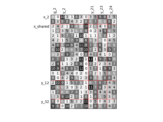
Twice as many variables

Or we can increase the size of each input and each output by a factor of 2.

names = input_names + list(discipline.get_output_data_names())
sizes = {name: dataset.sizes[name] * 2 for name in names}
scalable = create_scalable("ScalableDiagonalModel", dataset, sizes)
scalable.scalable_model.plot_dependency(save=False, show=False)

'None'

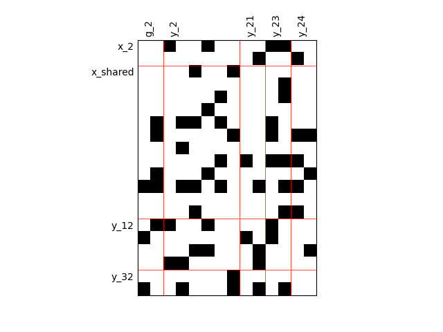
Binary IO dependencies

By default, any output component depends on any input component with a random level. We can also consider sparser input-output dependency by means of binary input-output dependency matrices. For that, we have to set the value of the fill factor which represents the part of connection between inputs and outputs. Then, a connection is represented by a black square while an absence of connection is presented by a white one. When the fill factor is equal to 1, any input is connected to any output. Conversely, when the fill factor is equal to 0, there is not a single connection between inputs and outputs.

Fill factor = 0.2

scalable = create_scalable("ScalableDiagonalModel", dataset, sizes, fill_factor=0.2)
scalable.scalable_model.plot_dependency(save=False, show=False)

'None'

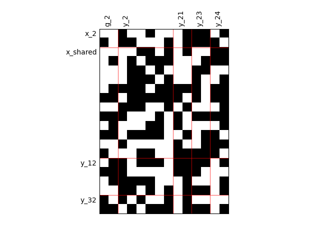
Fill factor = 0.5

scalable = create_scalable("ScalableDiagonalModel", dataset, sizes, fill_factor=0.5)
scalable.scalable_model.plot_dependency(save=False, show=False)

'None'

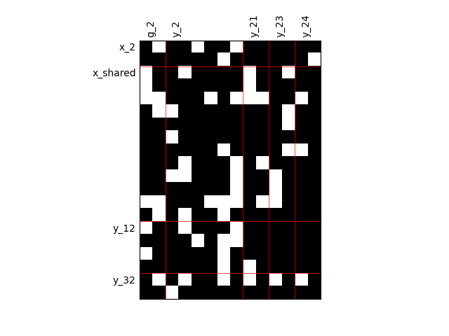
Fill factor = 0.8

scalable = create_scalable("ScalableDiagonalModel", dataset, sizes, fill_factor=0.8)
scalable.scalable_model.plot_dependency(save=False, show=False)

'None'

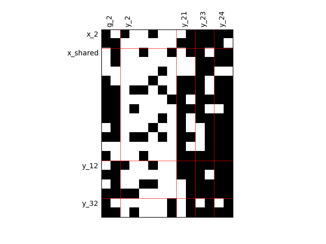
Heterogeneous dependencies

scalable = create_scalable(
    "ScalableDiagonalModel", dataset, sizes, fill_factor={"y_2": 0.2}
)
scalable.scalable_model.plot_dependency(save=False, show=False)

'None'

Group dependencies

scalable = create_scalable(
    "ScalableDiagonalModel", dataset, sizes, group_dep={"y_2": ["x_shared"]}
)
scalable.scalable_model.plot_dependency(save=False, show=False)
# Workaround for HTML rendering, instead of ``show=True``
plt.show()