Note
Click here to download the full example code
MDF-based MDO on the Sobieski SSBJ test case
from __future__ import annotations

from gemseo.api import configure_logger
from gemseo.api import create_discipline
from gemseo.api import create_scenario
from gemseo.api import generate_n2_plot
from gemseo.problems.sobieski.core.problem import SobieskiProblem

configure_logger()
<RootLogger root (INFO)>
Instantiate the disciplines
First, we instantiate the four disciplines of the use case:
SobieskiPropulsion,
SobieskiAerodynamics,
SobieskiMission
and SobieskiStructure.
disciplines = create_discipline(
    [
        "SobieskiPropulsion",
        "SobieskiAerodynamics",
        "SobieskiMission",
        "SobieskiStructure",
    ]
)
We can quickly access the most relevant information of any discipline (name, inputs,
and outputs) with Python’s print() function. Moreover, we can get the default
input values of a discipline with the attribute MDODiscipline.default_inputs
for discipline in disciplines:
    print(discipline)
    print(f"Default inputs: {discipline.default_inputs}")
SobieskiPropulsion
Default inputs: {'y_23': array([12562.01206488]), 'x_3': array([0.5]), 'x_shared': array([5.0e-02, 4.5e+04, 1.6e+00, 5.5e+00, 5.5e+01, 1.0e+03]), 'c_3': array([4360.])}
SobieskiAerodynamics
Default inputs: {'x_2': array([1.]), 'y_32': array([0.50279625]), 'x_shared': array([5.0e-02, 4.5e+04, 1.6e+00, 5.5e+00, 5.5e+01, 1.0e+03]), 'y_12': array([5.06069742e+04, 9.50000000e-01]), 'c_4': array([0.01375])}
SobieskiMission
Default inputs: {'y_14': array([50606.9741711 ,  7306.20262124]), 'x_shared': array([5.0e-02, 4.5e+04, 1.6e+00, 5.5e+00, 5.5e+01, 1.0e+03]), 'y_24': array([4.15006276]), 'y_34': array([1.10754577])}
SobieskiStructure
Default inputs: {'y_21': array([50606.9741711]), 'y_31': array([6354.32430691]), 'x_1': array([0.25, 1.  ]), 'x_shared': array([5.0e-02, 4.5e+04, 1.6e+00, 5.5e+00, 5.5e+01, 1.0e+03]), 'c_0': array([2000.]), 'c_1': array([25000.]), 'c_2': array([6.])}
You may also be interested in plotting the couplings of your disciplines.
A quick way of getting this information is the API function
generate_n2_plot(). A much more detailed explanation of coupling
visualization is available here.
generate_n2_plot(disciplines, save=False, show=True)

Build, execute and post-process the scenario
Then, we build the scenario which links the disciplines
with the formulation and the optimization algorithm. Here, we use the
MDF formulation. We tell the scenario to minimize -y_4 instead of
minimizing y_4 (range), which is the default option.
Instantiate the scenario
During the instantiation of the scenario, we provide some options for the MDF formulations:
formulation_options = {
    "tolerance": 1e-10,
    "max_mda_iter": 50,
    "warm_start": True,
    "use_lu_fact": True,
    "linear_solver_tolerance": 1e-15,
}
'warm_start: warm starts MDA,'warm_start: optimize the adjoints resolution by storing the Jacobian matrix LU factorization for the multiple RHS (objective + constraints). This saves CPU time if you can pay for the memory and have the full Jacobians available, not just matrix vector products.'linear_solver_tolerance': set the linear solver tolerance, idem we need full convergence
design_space = SobieskiProblem().design_space
print(design_space)
scenario = create_scenario(
    disciplines,
    "MDF",
    objective_name="y_4",
    design_space=design_space,
    maximize_objective=True,
    **formulation_options,
)
Design space:
+-------------+-------------+--------------------+-------------+-------+
| name        | lower_bound |       value        | upper_bound | type  |
+-------------+-------------+--------------------+-------------+-------+
| x_shared[0] |     0.01    |        0.05        |     0.09    | float |
| x_shared[1] |    30000    |       45000        |    60000    | float |
| x_shared[2] |     1.4     |        1.6         |     1.8     | float |
| x_shared[3] |     2.5     |        5.5         |     8.5     | float |
| x_shared[4] |      40     |         55         |      70     | float |
| x_shared[5] |     500     |        1000        |     1500    | float |
| x_1[0]      |     0.1     |        0.25        |     0.4     | float |
| x_1[1]      |     0.75    |         1          |     1.25    | float |
| x_2         |     0.75    |         1          |     1.25    | float |
| x_3         |     0.1     |        0.5         |      1      | float |
| y_14[0]     |    24850    |   50606.9741711    |    77100    | float |
| y_14[1]     |    -7700    |   7306.20262124    |    45000    | float |
| y_32        |    0.235    | 0.5027962499999999 |    0.795    | float |
| y_31        |     2960    |   6354.32430691    |    10185    | float |
| y_24        |     0.44    |     4.15006276     |    11.13    | float |
| y_34        |     0.44    |     1.10754577     |     1.98    | float |
| y_23        |     3365    |   12194.2671934    |    26400    | float |
| y_21        |    24850    |   50606.9741711    |    77250    | float |
| y_12[0]     |    24850    |     50606.9742     |    77250    | float |
| y_12[1]     |     0.45    |        0.95        |     1.5     | float |
+-------------+-------------+--------------------+-------------+-------+
Set the design constraints
for c_name in ["g_1", "g_2", "g_3"]:
    scenario.add_constraint(c_name, "ineq")
XDSMIZE the scenario
Generate the XDSM file on the fly, setting print_statuses=True
will print the status in the console
html_output (default True), will generate a self-contained
HTML file, that can be automatically open using open_browser=True
scenario.xdsmize()
INFO - 16:58:36: Generating HTML XDSM file in : xdsm.html
Define the algorithm inputs
We set the maximum number of iterations, the optimizer
and the optimizer options. Algorithm specific options are passed there.
Use get_algorithm_options_schema() API function for more
information or read the documentation.
Here ftol_rel option is a stop criteria based on the relative difference in the objective between two iterates ineq_tolerance the tolerance determination of the optimum; this is specific to the GEMSEO wrapping and not in the solver.
algo_options = {
    "ftol_rel": 1e-10,
    "ineq_tolerance": 2e-3,
    "normalize_design_space": True,
}
scn_inputs = {"max_iter": 10, "algo": "SLSQP", "algo_options": algo_options}
See also
We can also generate a backup file for the optimization,
as well as plots on the fly of the optimization history if option
generate_opt_plot is True.
This slows down a lot the process, here since SSBJ is very light
scenario.set_optimization_history_backup(file_path="mdf_backup.h5",
                                         each_new_iter=True,
                                         each_store=False, erase=True,
                                         pre_load=False,
                                         generate_opt_plot=True)
Execute the scenario
scenario.execute(scn_inputs)
    INFO - 16:58:36:
    INFO - 16:58:36: *** Start MDOScenario execution ***
    INFO - 16:58:36: MDOScenario
    INFO - 16:58:36:    Disciplines: SobieskiAerodynamics SobieskiMission SobieskiPropulsion SobieskiStructure
    INFO - 16:58:36:    MDO formulation: MDF
    INFO - 16:58:36: Optimization problem:
    INFO - 16:58:36:    minimize -y_4(x_shared, x_1, x_2, x_3) = -y_4(x_shared, x_1, x_2, x_3)
    INFO - 16:58:36:    with respect to x_1, x_2, x_3, x_shared
    INFO - 16:58:36:    subject to constraints:
    INFO - 16:58:36:       g_1(x_shared, x_1, x_2, x_3) <= 0.0
    INFO - 16:58:36:       g_2(x_shared, x_1, x_2, x_3) <= 0.0
    INFO - 16:58:36:       g_3(x_shared, x_1, x_2, x_3) <= 0.0
    INFO - 16:58:36:    over the design space:
    INFO - 16:58:36:    +-------------+-------------+-------+-------------+-------+
    INFO - 16:58:36:    | name        | lower_bound | value | upper_bound | type  |
    INFO - 16:58:36:    +-------------+-------------+-------+-------------+-------+
    INFO - 16:58:36:    | x_shared[0] |     0.01    |  0.05 |     0.09    | float |
    INFO - 16:58:36:    | x_shared[1] |    30000    | 45000 |    60000    | float |
    INFO - 16:58:36:    | x_shared[2] |     1.4     |  1.6  |     1.8     | float |
    INFO - 16:58:36:    | x_shared[3] |     2.5     |  5.5  |     8.5     | float |
    INFO - 16:58:36:    | x_shared[4] |      40     |   55  |      70     | float |
    INFO - 16:58:36:    | x_shared[5] |     500     |  1000 |     1500    | float |
    INFO - 16:58:36:    | x_1[0]      |     0.1     |  0.25 |     0.4     | float |
    INFO - 16:58:36:    | x_1[1]      |     0.75    |   1   |     1.25    | float |
    INFO - 16:58:36:    | x_2         |     0.75    |   1   |     1.25    | float |
    INFO - 16:58:36:    | x_3         |     0.1     |  0.5  |      1      | float |
    INFO - 16:58:36:    +-------------+-------------+-------+-------------+-------+
    INFO - 16:58:36: Solving optimization problem with algorithm SLSQP:
    INFO - 16:58:36: ...   0%|          | 0/10 [00:00<?, ?it]
    INFO - 16:58:36: ...  10%|█         | 1/10 [00:00<00:00, 10.56 it/sec, obj=-536]
    INFO - 16:58:36: ...  20%|██        | 2/10 [00:00<00:00, 10.78 it/sec, obj=-2.12e+3]
    INFO - 16:58:36: ...  30%|███       | 3/10 [00:00<00:00,  8.91 it/sec, obj=-3.64e+3]
    INFO - 16:58:36: ...  40%|████      | 4/10 [00:00<00:00,  9.35 it/sec, obj=-4.01e+3]
    INFO - 16:58:37: ...  50%|█████     | 5/10 [00:00<00:00,  8.92 it/sec, obj=-4.51e+3]
 WARNING - 16:58:37: Optimization found no feasible point !  The least infeasible point is selected.
    INFO - 16:58:37: Optimization result:
    INFO - 16:58:37:    Optimizer info:
    INFO - 16:58:37:       Status: 8
    INFO - 16:58:37:       Message: Positive directional derivative for linesearch
    INFO - 16:58:37:       Number of calls to the objective function by the optimizer: 6
    INFO - 16:58:37:    Solution:
 WARNING - 16:58:37:       The solution is not feasible.
    INFO - 16:58:37:       Objective: -3643.2646614710907
    INFO - 16:58:37:       Standardized constraints:
    INFO - 16:58:37:          g_1 = [-0.02648406 -0.03933265 -0.04887821 -0.05560436 -0.06050463 -0.13630937
    INFO - 16:58:37:  -0.10369063]
    INFO - 16:58:37:          g_2 = 0.002396186936539646
    INFO - 16:58:37:          g_3 = [-0.50236422 -0.49763578 -0.23179683 -0.18266046]
    INFO - 16:58:37:       Design space:
    INFO - 16:58:37:       +-------------+-------------+---------------------+-------------+-------+
    INFO - 16:58:37:       | name        | lower_bound |        value        | upper_bound | type  |
    INFO - 16:58:37:       +-------------+-------------+---------------------+-------------+-------+
    INFO - 16:58:37:       | x_shared[0] |     0.01    | 0.06059904673413494 |     0.09    | float |
    INFO - 16:58:37:       | x_shared[1] |    30000    |        60000        |    60000    | float |
    INFO - 16:58:37:       | x_shared[2] |     1.4     |   1.40455692827199  |     1.8     | float |
    INFO - 16:58:37:       | x_shared[3] |     2.5     |         2.5         |     8.5     | float |
    INFO - 16:58:37:       | x_shared[4] |      40     |          70         |      70     | float |
    INFO - 16:58:37:       | x_shared[5] |     500     |         1500        |     1500    | float |
    INFO - 16:58:37:       | x_1[0]      |     0.1     |  0.3947569275200153 |     0.4     | float |
    INFO - 16:58:37:       | x_1[1]      |     0.75    |         0.75        |     1.25    | float |
    INFO - 16:58:37:       | x_2         |     0.75    |         0.75        |     1.25    | float |
    INFO - 16:58:37:       | x_3         |     0.1     |  0.1205118700740507 |      1      | float |
    INFO - 16:58:37:       +-------------+-------------+---------------------+-------------+-------+
    INFO - 16:58:37: *** End MDOScenario execution (time: 0:00:00.596875) ***

{'max_iter': 10, 'algo': 'SLSQP', 'algo_options': {'ftol_rel': 1e-10, 'ineq_tolerance': 0.002, 'normalize_design_space': True}}
Save the optimization history
We can save the whole optimization problem and its history for further post processing:
scenario.save_optimization_history("mdf_history.h5", file_format="hdf5")
INFO - 16:58:37: Export optimization problem to file: mdf_history.h5
We can also save only calls to functions and design variables history:
scenario.save_optimization_history("mdf_history.xml", file_format="ggobi")
INFO - 16:58:37: Export to ggobi for functions: ['-y_4', 'Iter', 'g_1', 'g_2', 'g_3']
INFO - 16:58:37: Export to ggobi file: mdf_history.xml
Print optimization metrics
scenario.print_execution_metrics()
INFO - 16:58:37: Scenario Execution Statistics
INFO - 16:58:37:    Discipline: SobieskiPropulsion
INFO - 16:58:37:       Executions number: 95
INFO - 16:58:37:       Execution time: 0.030784266999035026 s
INFO - 16:58:37:       Linearizations number: 5
INFO - 16:58:37:    Discipline: SobieskiAerodynamics
INFO - 16:58:37:       Executions number: 101
INFO - 16:58:37:       Execution time: 0.07054826000421599 s
INFO - 16:58:37:       Linearizations number: 5
INFO - 16:58:37:    Discipline: SobieskiMission
INFO - 16:58:37:       Executions number: 5
INFO - 16:58:37:       Execution time: 0.00046418100100709125 s
INFO - 16:58:37:       Linearizations number: 5
INFO - 16:58:37:    Discipline: SobieskiStructure
INFO - 16:58:37:       Executions number: 101
INFO - 16:58:37:       Execution time: 0.14226223899913748 s
INFO - 16:58:37:       Linearizations number: 5
INFO - 16:58:37:    Total number of executions calls: 302
INFO - 16:58:37:    Total number of linearizations: 20
Post-process the results
Plot the optimization history view
scenario.post_process("OptHistoryView", save=False, show=True)

 WARNING - 16:58:37: Optimization found no feasible point !  The least infeasible point is selected.

<gemseo.post.opt_history_view.OptHistoryView object at 0x7fbc39c21370>
Plot the basic history view
scenario.post_process(
    "BasicHistory", variable_names=["x_shared"], save=False, show=True
)
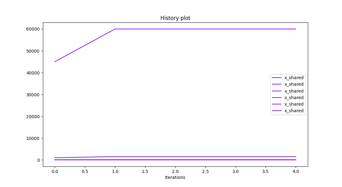
<gemseo.post.basic_history.BasicHistory object at 0x7fbc4408da90>
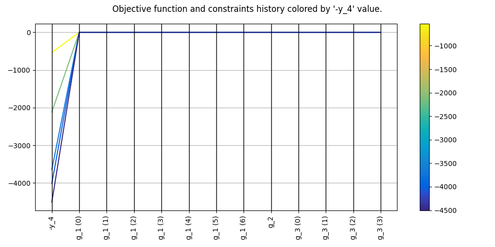
Plot the constraints and objective history
scenario.post_process("ObjConstrHist", save=False, show=True)
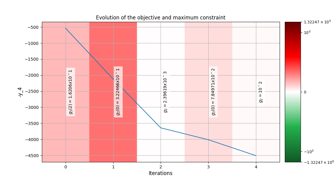
<gemseo.post.obj_constr_hist.ObjConstrHist object at 0x7fbc3986e130>
Plot the constraints history
scenario.post_process(
    "ConstraintsHistory",
    constraint_names=["g_1", "g_2", "g_3"],
    save=False,
    show=True,
)
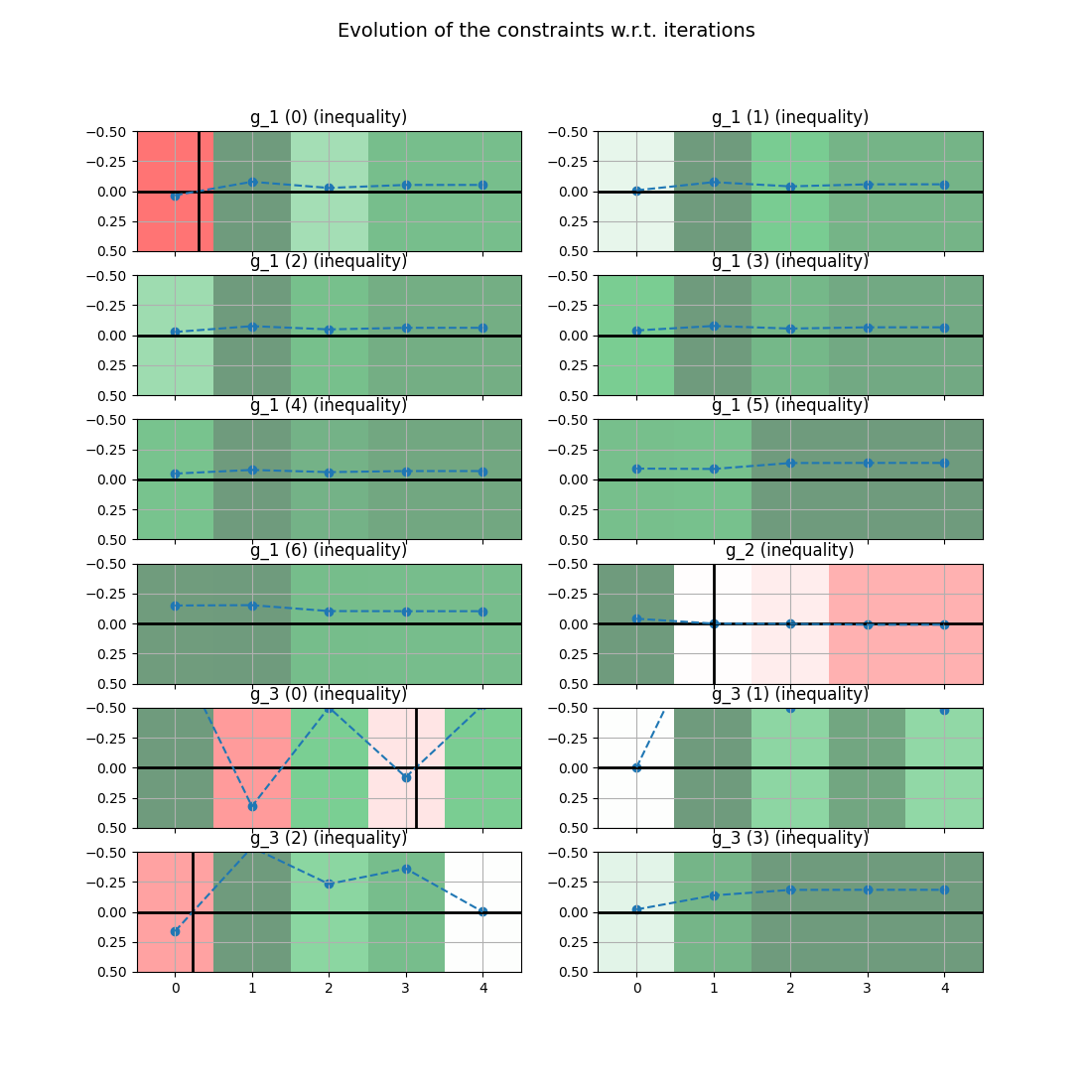
<gemseo.post.constraints_history.ConstraintsHistory object at 0x7fbc39dd5790>
Plot the constraints history using a radar chart
scenario.post_process(
    "RadarChart",
    constraint_names=["g_1", "g_2", "g_3"],
    save=False,
    show=True,
)
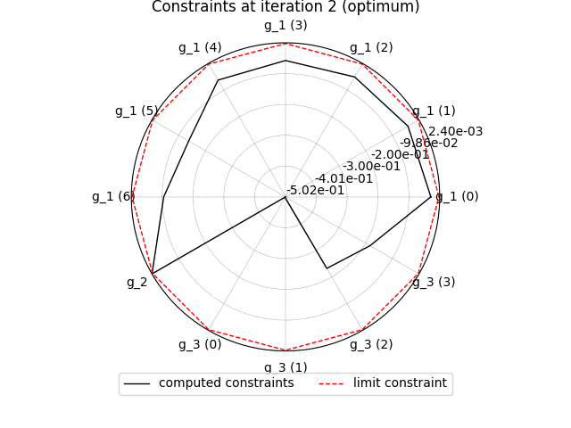
<gemseo.post.radar_chart.RadarChart object at 0x7fbc4404a940>
Plot the quadratic approximation of the objective
scenario.post_process("QuadApprox", function="-y_4", save=False, show=True)

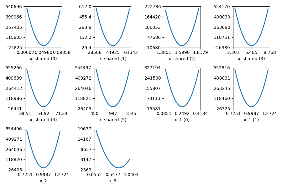
<gemseo.post.quad_approx.QuadApprox object at 0x7fbc561f0e80>
Plot the functions using a SOM
scenario.post_process("SOM", save=False, show=True)
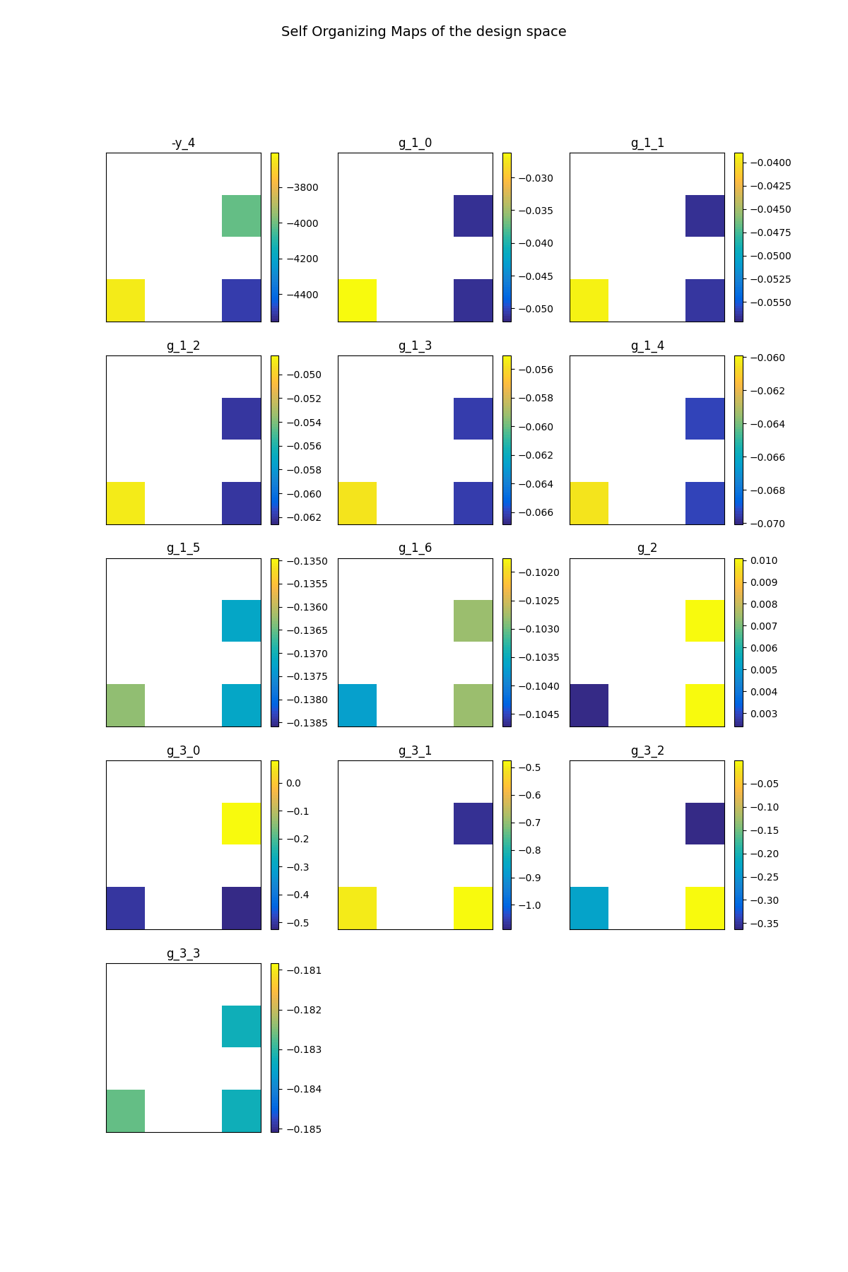
    INFO - 16:58:40: Building Self Organizing Map from optimization history:
    INFO - 16:58:40:     Number of neurons in x direction = 4
    INFO - 16:58:40:     Number of neurons in y direction = 4

<gemseo.post.som.SOM object at 0x7fbc44089520>
Plot the scatter matrix of variables of interest
scenario.post_process(
    "ScatterPlotMatrix",
    variable_names=["-y_4", "g_1"],
    save=False,
    show=True,
    fig_size=(14, 14),
)
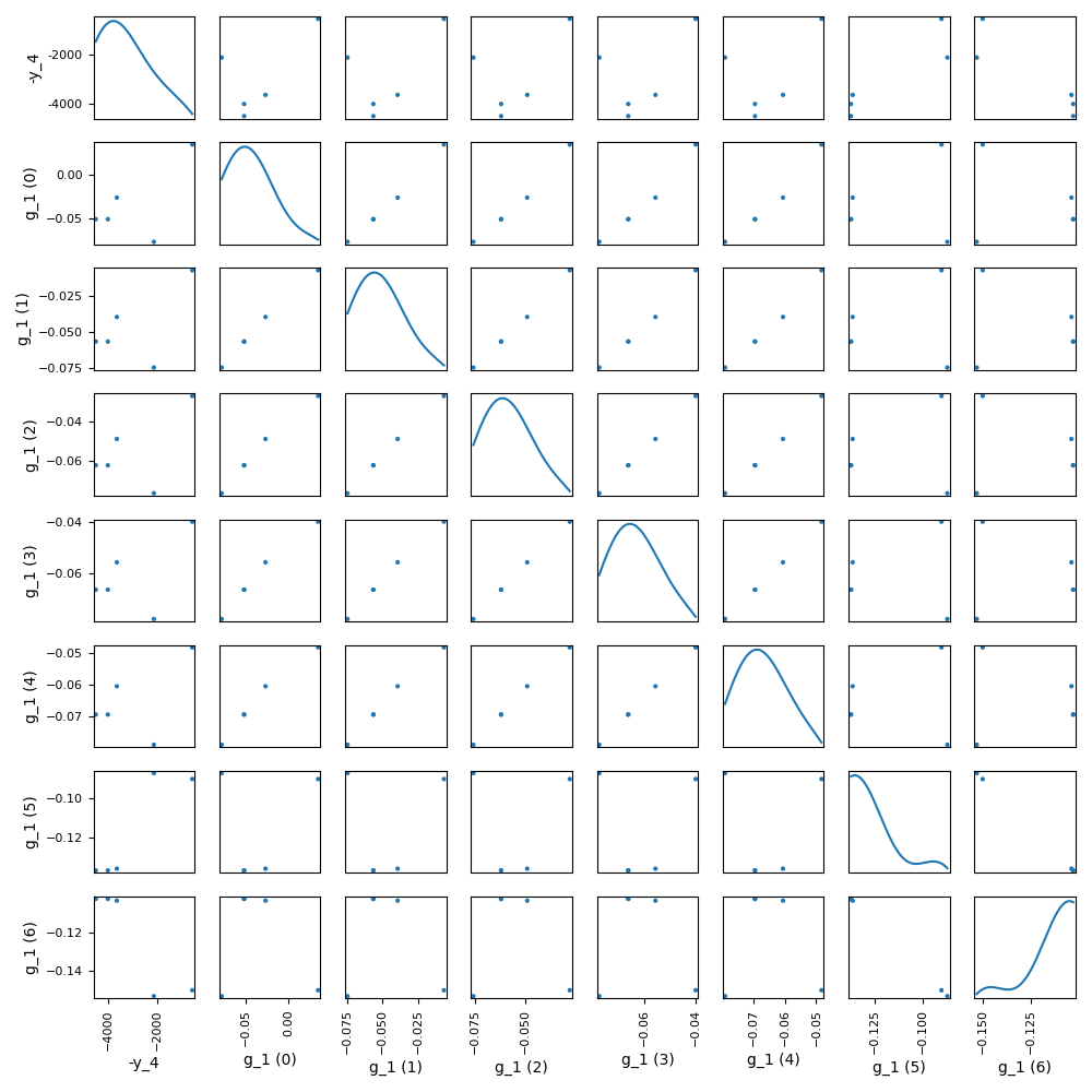
<gemseo.post.scatter_mat.ScatterPlotMatrix object at 0x7fbc6b1b3730>
Plot the variables using the parallel coordinates
scenario.post_process("ParallelCoordinates", save=False, show=True)
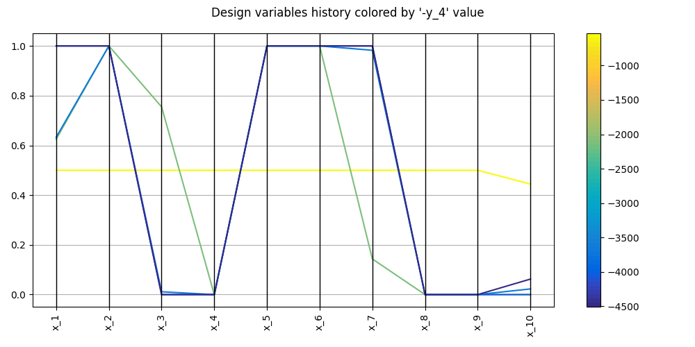
<gemseo.post.para_coord.ParallelCoordinates object at 0x7fbc558b8a30>
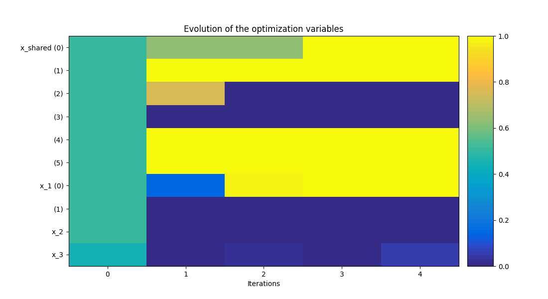
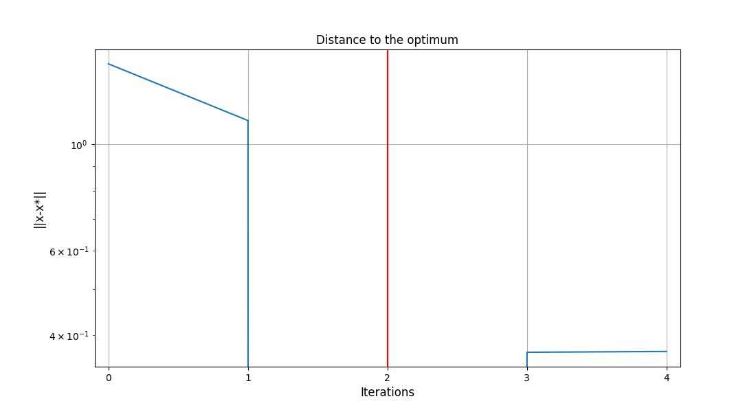
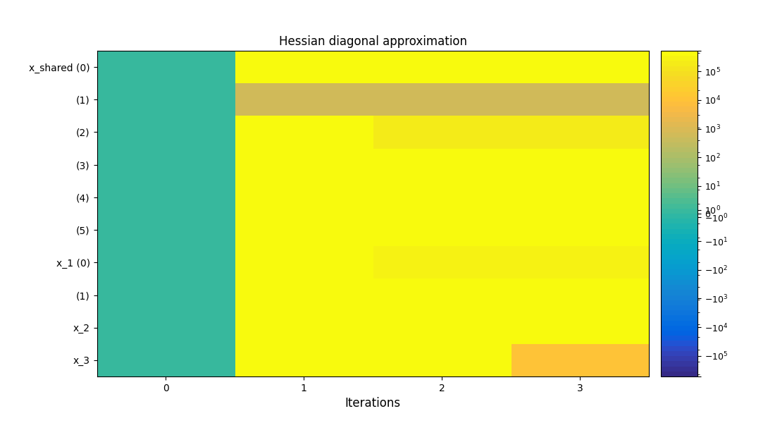
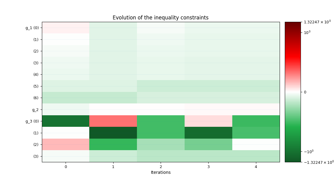
Plot the robustness of the solution
scenario.post_process("Robustness", save=True, show=True)
<gemseo.post.robustness.Robustness object at 0x7fbc37a8da60>
Plot the influence of the design variables
scenario.post_process("VariableInfluence", fig_size=(14, 14), save=False, show=True)
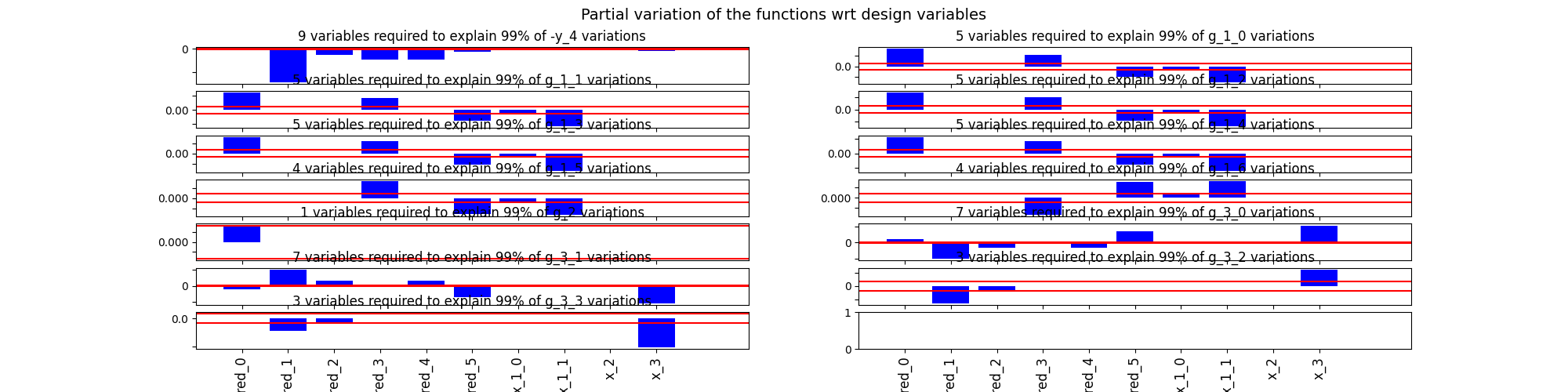
 WARNING - 16:58:45: Optimization found no feasible point !  The least infeasible point is selected.
    INFO - 16:58:45: VariableInfluence for function -y_4
    INFO - 16:58:45: Most influential variables indices to explain % of the function variation: 99
    INFO - 16:58:45: [1 4 3 2 5 9 7 8 0]
/home/docs/checkouts/readthedocs.org/user_builds/gemseo/envs/4.3.0.post0/lib/python3.9/site-packages/gemseo/post/variable_influence.py:230: UserWarning: FixedFormatter should only be used together with FixedLocator
  axe.set_xticklabels(x_labels, fontsize=font_size, rotation=rotation)
    INFO - 16:58:45: VariableInfluence for function g_1_0
    INFO - 16:58:45: Most influential variables indices to explain % of the function variation: 99
    INFO - 16:58:45: [0 7 3 5 6]
    INFO - 16:58:45: VariableInfluence for function g_1_1
    INFO - 16:58:45: Most influential variables indices to explain % of the function variation: 99
    INFO - 16:58:45: [0 7 3 5 6]
    INFO - 16:58:45: VariableInfluence for function g_1_2
    INFO - 16:58:45: Most influential variables indices to explain % of the function variation: 99
    INFO - 16:58:45: [7 0 3 5 6]
    INFO - 16:58:45: VariableInfluence for function g_1_3
    INFO - 16:58:45: Most influential variables indices to explain % of the function variation: 99
    INFO - 16:58:45: [7 0 3 5 6]
    INFO - 16:58:45: VariableInfluence for function g_1_4
    INFO - 16:58:45: Most influential variables indices to explain % of the function variation: 99
    INFO - 16:58:45: [7 0 3 5 6]
    INFO - 16:58:45: VariableInfluence for function g_1_5
    INFO - 16:58:45: Most influential variables indices to explain % of the function variation: 99
    INFO - 16:58:45: [3 7 5 6]
    INFO - 16:58:45: VariableInfluence for function g_1_6
    INFO - 16:58:45: Most influential variables indices to explain % of the function variation: 99
    INFO - 16:58:45: [3 7 5 6]
    INFO - 16:58:45: VariableInfluence for function g_2
    INFO - 16:58:45: Most influential variables indices to explain % of the function variation: 99
    INFO - 16:58:45: [0]
    INFO - 16:58:45: VariableInfluence for function g_3_0
    INFO - 16:58:45: Most influential variables indices to explain % of the function variation: 99
    INFO - 16:58:45: [9 1 5 2 4 0 8]
    INFO - 16:58:46: VariableInfluence for function g_3_1
    INFO - 16:58:46: Most influential variables indices to explain % of the function variation: 99
    INFO - 16:58:46: [9 1 5 2 4 0 8]
    INFO - 16:58:46: VariableInfluence for function g_3_2
    INFO - 16:58:46: Most influential variables indices to explain % of the function variation: 99
    INFO - 16:58:46: [1 9 2]
    INFO - 16:58:46: VariableInfluence for function g_3_3
    INFO - 16:58:46: Most influential variables indices to explain % of the function variation: 99
    INFO - 16:58:46: [9 1 2]

<gemseo.post.variable_influence.VariableInfluence object at 0x7fbc6b1c8250>
Total running time of the script: ( 0 minutes 10.355 seconds)