Note
Click here to download the full example code
Quadratic approximations
In this example, we illustrate the use of the QuadApprox plot
on the Sobieski’s SSBJ problem.
from __future__ import annotations

from gemseo.api import configure_logger
from gemseo.api import create_discipline
from gemseo.api import create_scenario
from gemseo.problems.sobieski.core.problem import SobieskiProblem
Import
The first step is to import some functions from the API and a method to get the design space.
configure_logger()
<RootLogger root (INFO)>
Description
The QuadApprox post-processing
performs a quadratic approximation of a given function
from an optimization history
and plot the results as cuts of the approximation.
Create disciplines
Then, we instantiate the disciplines of the Sobieski’s SSBJ problem: Propulsion, Aerodynamics, Structure and Mission
disciplines = create_discipline(
    [
        "SobieskiPropulsion",
        "SobieskiAerodynamics",
        "SobieskiStructure",
        "SobieskiMission",
    ]
)
Create design space
We also read the design space from the SobieskiProblem.
design_space = SobieskiProblem().design_space
Create and execute scenario
The next step is to build an MDO scenario in order to maximize the range, encoded ‘y_4’, with respect to the design parameters, while satisfying the inequality constraints ‘g_1’, ‘g_2’ and ‘g_3’. We can use the MDF formulation, the SLSQP optimization algorithm and a maximum number of iterations equal to 100.
scenario = create_scenario(
    disciplines,
    formulation="MDF",
    objective_name="y_4",
    maximize_objective=True,
    design_space=design_space,
)
scenario.set_differentiation_method()
for constraint in ["g_1", "g_2", "g_3"]:
    scenario.add_constraint(constraint, "ineq")
scenario.execute({"algo": "SLSQP", "max_iter": 10})
    INFO - 16:55:34:
    INFO - 16:55:34: *** Start MDOScenario execution ***
    INFO - 16:55:34: MDOScenario
    INFO - 16:55:34:    Disciplines: SobieskiAerodynamics SobieskiMission SobieskiPropulsion SobieskiStructure
    INFO - 16:55:34:    MDO formulation: MDF
    INFO - 16:55:34: Optimization problem:
    INFO - 16:55:34:    minimize -y_4(x_shared, x_1, x_2, x_3) = -y_4(x_shared, x_1, x_2, x_3)
    INFO - 16:55:34:    with respect to x_1, x_2, x_3, x_shared
    INFO - 16:55:34:    subject to constraints:
    INFO - 16:55:34:       g_1(x_shared, x_1, x_2, x_3) <= 0.0
    INFO - 16:55:34:       g_2(x_shared, x_1, x_2, x_3) <= 0.0
    INFO - 16:55:34:       g_3(x_shared, x_1, x_2, x_3) <= 0.0
    INFO - 16:55:34:    over the design space:
    INFO - 16:55:34:    +-------------+-------------+-------+-------------+-------+
    INFO - 16:55:34:    | name        | lower_bound | value | upper_bound | type  |
    INFO - 16:55:34:    +-------------+-------------+-------+-------------+-------+
    INFO - 16:55:34:    | x_shared[0] |     0.01    |  0.05 |     0.09    | float |
    INFO - 16:55:34:    | x_shared[1] |    30000    | 45000 |    60000    | float |
    INFO - 16:55:34:    | x_shared[2] |     1.4     |  1.6  |     1.8     | float |
    INFO - 16:55:34:    | x_shared[3] |     2.5     |  5.5  |     8.5     | float |
    INFO - 16:55:34:    | x_shared[4] |      40     |   55  |      70     | float |
    INFO - 16:55:34:    | x_shared[5] |     500     |  1000 |     1500    | float |
    INFO - 16:55:34:    | x_1[0]      |     0.1     |  0.25 |     0.4     | float |
    INFO - 16:55:34:    | x_1[1]      |     0.75    |   1   |     1.25    | float |
    INFO - 16:55:34:    | x_2         |     0.75    |   1   |     1.25    | float |
    INFO - 16:55:34:    | x_3         |     0.1     |  0.5  |      1      | float |
    INFO - 16:55:34:    +-------------+-------------+-------+-------------+-------+
    INFO - 16:55:34: Solving optimization problem with algorithm SLSQP:
    INFO - 16:55:34: ...   0%|          | 0/10 [00:00<?, ?it]
    INFO - 16:55:34: ...  10%|█         | 1/10 [00:00<00:00, 11.40 it/sec, obj=-536]
    INFO - 16:55:34: ...  20%|██        | 2/10 [00:00<00:00,  8.87 it/sec, obj=-2.12e+3]
 WARNING - 16:55:34: MDAJacobi has reached its maximum number of iterations but the normed residual 1.4486313079508508e-06 is still above the tolerance 1e-06.
    INFO - 16:55:34: ...  30%|███       | 3/10 [00:00<00:00,  7.69 it/sec, obj=-3.75e+3]
    INFO - 16:55:34: ...  40%|████      | 4/10 [00:00<00:00,  7.51 it/sec, obj=-4.01e+3]
 WARNING - 16:55:34: MDAJacobi has reached its maximum number of iterations but the normed residual 2.928004141058104e-06 is still above the tolerance 1e-06.
    INFO - 16:55:34: ...  50%|█████     | 5/10 [00:00<00:00,  7.16 it/sec, obj=-4.49e+3]
    INFO - 16:55:34: ...  60%|██████    | 6/10 [00:00<00:00,  7.29 it/sec, obj=-3.4e+3]
    INFO - 16:55:34: ...  70%|███████   | 7/10 [00:00<00:00,  7.91 it/sec, obj=-4.93e+3]
    INFO - 16:55:35: ...  80%|████████  | 8/10 [00:00<00:00,  8.25 it/sec, obj=-4.76e+3]
    INFO - 16:55:35: ...  90%|█████████ | 9/10 [00:01<00:00,  8.58 it/sec, obj=-4.62e+3]
    INFO - 16:55:35: ... 100%|██████████| 10/10 [00:01<00:00,  8.95 it/sec, obj=-4.56e+3]
    INFO - 16:55:35: Optimization result:
    INFO - 16:55:35:    Optimizer info:
    INFO - 16:55:35:       Status: None
    INFO - 16:55:35:       Message: Maximum number of iterations reached. GEMSEO Stopped the driver
    INFO - 16:55:35:       Number of calls to the objective function by the optimizer: 12
    INFO - 16:55:35:    Solution:
    INFO - 16:55:35:       The solution is feasible.
    INFO - 16:55:35:       Objective: -3749.8868975554387
    INFO - 16:55:35:       Standardized constraints:
    INFO - 16:55:35:          g_1 = [-0.01671296 -0.03238836 -0.04350867 -0.05123129 -0.05681738 -0.13780658
    INFO - 16:55:35:  -0.10219342]
    INFO - 16:55:35:          g_2 = -0.0004062839430756249
    INFO - 16:55:35:          g_3 = [-0.66482546 -0.33517454 -0.11023156 -0.183255  ]
    INFO - 16:55:35:       Design space:
    INFO - 16:55:35:       +-------------+-------------+---------------------+-------------+-------+
    INFO - 16:55:35:       | name        | lower_bound |        value        | upper_bound | type  |
    INFO - 16:55:35:       +-------------+-------------+---------------------+-------------+-------+
    INFO - 16:55:35:       | x_shared[0] |     0.01    | 0.05989842901423112 |     0.09    | float |
    INFO - 16:55:35:       | x_shared[1] |    30000    |  59853.73840058666  |    60000    | float |
    INFO - 16:55:35:       | x_shared[2] |     1.4     |         1.4         |     1.8     | float |
    INFO - 16:55:35:       | x_shared[3] |     2.5     |  2.527371250092273  |     8.5     | float |
    INFO - 16:55:35:       | x_shared[4] |      40     |  69.86825198198687  |      70     | float |
    INFO - 16:55:35:       | x_shared[5] |     500     |  1495.734648986894  |     1500    | float |
    INFO - 16:55:35:       | x_1[0]      |     0.1     |         0.4         |     0.4     | float |
    INFO - 16:55:35:       | x_1[1]      |     0.75    |  0.7521124139939552 |     1.25    | float |
    INFO - 16:55:35:       | x_2         |     0.75    |  0.7520888531444992 |     1.25    | float |
    INFO - 16:55:35:       | x_3         |     0.1     |  0.1398000762238233 |      1      | float |
    INFO - 16:55:35:       +-------------+-------------+---------------------+-------------+-------+
    INFO - 16:55:35: *** End MDOScenario execution (time: 0:00:01.134528) ***

{'max_iter': 10, 'algo': 'SLSQP'}
Post-process scenario
Lastly, we post-process the scenario by means of the QuadApprox
plot which performs a quadratic approximation of a given function
from an optimization history and plot the results as cuts of the
approximation.
Tip
Each post-processing method requires different inputs and offers a variety
of customization options. Use the API function
get_post_processing_options_schema() to print a table with
the options for any post-processing algorithm.
Or refer to our dedicated page:
Post-processing algorithms.
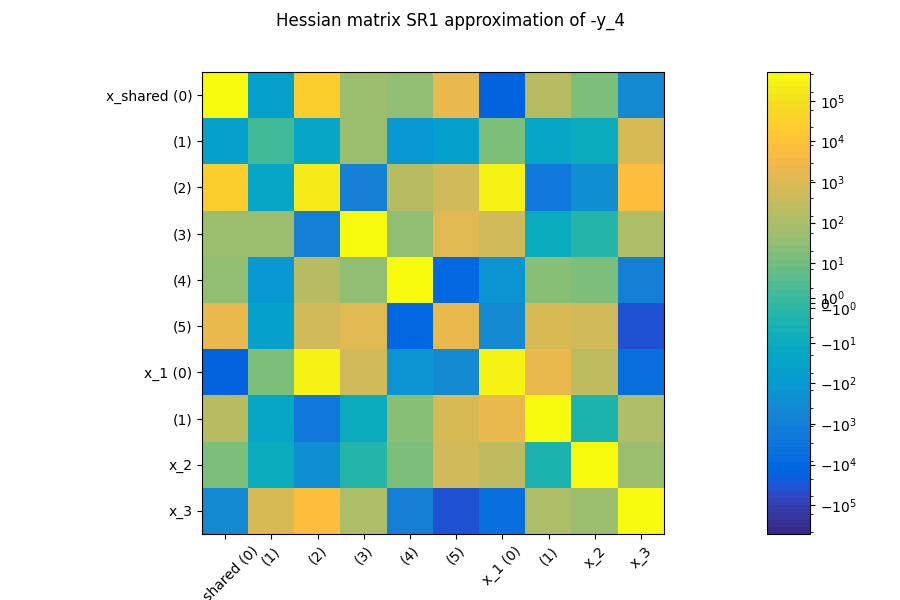
The first plot shows an approximation of the Hessian matrix \(\frac{\partial^2 f}{\partial x_i \partial x_j}\) based on the Symmetric Rank 1 method (SR1) [NW06]. The color map uses a symmetric logarithmic (symlog) scale. This plots the cross influence of the design variables on the objective function or constraints. For instance, on the last figure, the maximal second-order sensitivity is \(\frac{\partial^2 -y_4}{\partial^2 x_0} = 2.10^5\), which means that the \(x_0\) is the most influential variable. Then, the cross derivative \(\frac{\partial^2 -y_4}{\partial x_0 \partial x_2} = 5.10^4\) is positive and relatively high compared to the previous one but the combined effects of \(x_0\) and \(x_2\) are non-negligible in comparison.
scenario.post_process("QuadApprox", function="-y_4", save=False, show=True)
<gemseo.post.quad_approx.QuadApprox object at 0x7fbc56179dc0>
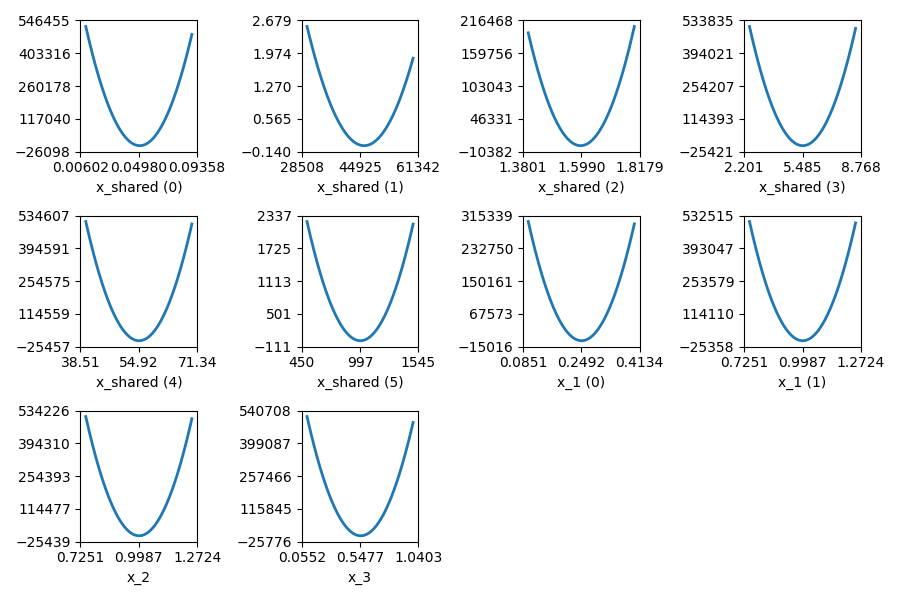
The second plot represents the quadratic approximation of the objective around the optimal solution : \(a_{i}(t)=0.5 (t-x^*_i)^2 \frac{\partial^2 f}{\partial x_i^2} + (t-x^*_i) \frac{\partial f}{\partial x_i} + f(x^*)\), where \(x^*\) is the optimal solution. This approximation highlights the sensitivity of the objective function with respect to the design variables: we notice that the design variables \(x\_1, x\_5, x\_6\) have little influence , whereas \(x\_0, x\_2, x\_9\) have a huge influence on the objective. This trend is also noted in the diagonal terms of the Hessian matrix \(\frac{\partial^2 f}{\partial x_i^2}\).
Total running time of the script: ( 0 minutes 1.896 seconds)