van_der_pol module¶

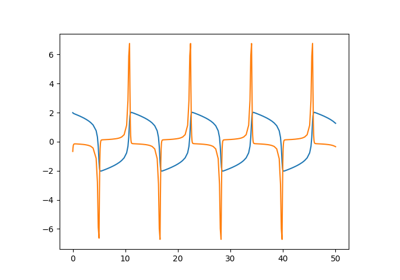
The Van der Pol (VDP) problem describing an oscillator with non-linear damping.

Van der Pol, B. & Van Der Mark, J. Frequency Demultiplication. Nature 120, 363-364 (1927).

The Van der Pol problem is written as follows:

\[\frac{d^2 x(t)}{dt^2} - \mu (1-x(t)^2) \frac{dx(t)}{dt} + x = 0\]

where \(x(t)\) is the position coordinate as a function of time, and \(\mu\) is a scalar parameter indicating the stiffness.

This problem can be rewrittent in a 2-dimensional form with only first-order derivatives. Let \(y = \frac{dx}{dt}\) and \(s = \begin{pmatrix}x\\y\end{pmatrix}\). Then the Van der Pol problem is:

\[\frac{ds}{dt} = f(s, t)\]

with

\[\begin{split}f : s = \begin{pmatrix} x \\ y \end{pmatrix} \mapsto \begin{pmatrix} y \\ \mu (1-x^2) y - x \end{pmatrix}\end{split}\]

The jacobian of this function can be expressed analytically:

\[\begin{split}\mathrm{Jac}\, f = \begin{pmatrix} 0 & 1 \\ -2\mu xy - 1 & \mu (1 - x^2) \end{pmatrix}\end{split}\]

There is no exact solution to the Van der Pol oscillator problem in terms of known tabulated functions (see Panayotounakos et al., On the Lack of Analytic Solutions of the Van Der Pol Oscillator. ZAMM 83, nᵒ 9 (1 septembre 2003)).

class gemseo.problems.ode.van_der_pol.VanDerPol(initial_time=0, final_time=0.5, mu=1000.0, use_jacobian=True, state_vector=None)[source]¶

Bases: ODEProblem

Representation of an oscillator with non-linear damping.

Parameters:

mu (float) –
The stiffness parameter.

By default it is set to 1000.0.
initial_time (float) –
The start of the integration interval.

By default it is set to 0.
final_time (float) –
The end of the integration interval.

By default it is set to 0.5.
use_jacobian (bool) –
Whether to use the analytical expression of the Jacobian. If false, use finite differences to estimate the Jacobian.

By default it is set to True.
state_vector (NDArray[float]) – The state vector of the system.

check()¶

Ensure the parameters of the problem are consistent.

Raises:: ValueError – If the state and time shapes are inconsistent.
Return type:: None

check_jacobian(state_vector, approximation_mode=ApproximationMode.FINITE_DIFFERENCES, step=1e-06, error_max=1e-08)¶

Check if the Jacobian function is correct.

At a given state, compare the value of the Jacobian computed by the function provided by ther user to an approximated value computed by finite-differences for example.

Parameters:

state_vector (ArrayLike) – The state at which the Jacobian is checked.
approximation_mode (ApproximationMode) –
The approximation mode.

By default it is set to “finite_differences”.
step (float) –
The step used to approximate the gradients.

By default it is set to 1e-06.
error_max (float) –
The error threshold above which the Jacobian is deemed to be incorrect.

By default it is set to 1e-08.

Raises:

ValueError – When the Jacobian function is wrong.

Return type:

None

adjoint_wrt_desvar: NumberArray¶: The adjoint of the problem relative to the design variables.

adjoint_wrt_state: NumberArray¶: The adjoint of the problem relative to the state.

initial_state: NumberArray¶: The initial conditions \((t_0,s_0)\) of the ODE.

integration_interval: tuple[float, float]¶: The interval of integration.

jac: Callable[[float, NumberArray], NumberArray] | NumberArray | None¶

The function to compute the Jacobian of \(f\).

If Callable, the Jacobian is assumed to be dependent on time and state. It will be called as jac(time, state) as necessary. If NumberArray, the Jacobian is assumed to be constant. If None, the Jacobian will be approximated by finite differences.

jac_desvar: Callable[[float, NumberArray], NumberArray]¶: The function to compute the Jacobian of \(f\) relative to the design variables.

result: ODEResult¶: The result of the ODE problem.

rhs_function: Callable[[float, NumberArray], NumberArray]¶: The function \(f\).

state_vect: NDArray[float]¶: State vector \(s=(x, \dot{x})\) of the system.

property time_vector¶: The times at which the solution shall be evaluated.

Examples using VanDerPol¶

Solve an ODE: the Van der Pol problem