gemseo / uncertainty / sensitivity / correlation

analysis module¶

Class for the estimation of various correlation coefficients.

class gemseo.uncertainty.sensitivity.correlation.analysis.CorrelationAnalysis(disciplines, parameter_space, n_samples, output_names=(), algo='', algo_options=mappingproxy({}), formulation='MDF', **formulation_options)[source]

Bases: BaseSensitivityAnalysis

Sensitivity analysis based on indices using correlation measures.

Examples

>>> from numpy import pi
>>> from gemseo import create_discipline, create_parameter_space
>>> from gemseo.uncertainty.sensitivity.correlation.analysis import (
...     CorrelationAnalysis,
... )
>>>
>>> expressions = {"y": "sin(x1)+7*sin(x2)**2+0.1*x3**4*sin(x1)"}
>>> discipline = create_discipline(
...     "AnalyticDiscipline", expressions=expressions
... )
>>>
>>> parameter_space = create_parameter_space()
>>> parameter_space.add_random_variable(
...     "x1", "OTUniformDistribution", minimum=-pi, maximum=pi
... )
>>> parameter_space.add_random_variable(
...     "x2", "OTUniformDistribution", minimum=-pi, maximum=pi
... )
>>> parameter_space.add_random_variable(
...     "x3", "OTUniformDistribution", minimum=-pi, maximum=pi
... )
>>>
>>> analysis = CorrelationAnalysis(
...     [discipline], parameter_space, n_samples=1000
... )
>>> indices = analysis.compute_indices()

Parameters:

disciplines (Collection[MDODiscipline]) – The discipline or disciplines to use for the analysis.
parameter_space (ParameterSpace) – A parameter space.
n_samples (int) – A number of samples. If None, the number of samples is computed by the algorithm.
output_names (Iterable[str]) –
The disciplines’ outputs to be considered for the analysis. If empty, use all the outputs.

By default it is set to ().
algo (str) –
The name of the DOE algorithm. If empty, use the BaseSensitivityAnalysis.DEFAULT_DRIVER.

By default it is set to “”.
algo_options (Mapping[str, DOELibraryOptionType]) –
The options of the DOE algorithm.

By default it is set to {}.
formulation (str) –
The name of the MDOFormulation to sample the disciplines.

By default it is set to “MDF”.
**formulation_options (Any) – The options of the MDOFormulation.

class Method(value)[source]

Bases: StrEnum

The names of the sensitivity methods.

KENDALL = 'Kendall': The Kendall rank correlation coefficient.

PCC = 'PCC': The partial correlation coefficient.

PEARSON = 'Pearson': The Pearson coefficient.

PRCC = 'PRCC': The partial rank correlation coefficient.

SPEARMAN = 'Spearman': The Spearman coefficient.

SRC = 'SRC': The standard regression coefficient.

SRRC = 'SRRC': The standard rank regression coefficient.

SSRC = 'SSRC': The squared standard regression coefficient.

compute_indices(outputs=())[source]

Compute the sensitivity indices.

Parameters:

outputs (str | Sequence[str]) –

The name(s) of the output(s) for which to compute the sensitivity indices. If empty, use the names of the outputs set at instantiation.

By default it is set to ().

Returns:

The sensitivity indices.

With the following structure:

{
    "method_name": {
        "output_name": [
            {
                "input_name": data_array,
            }
        ]
    }
}

Return type:

dict[str, FirstOrderIndicesType]

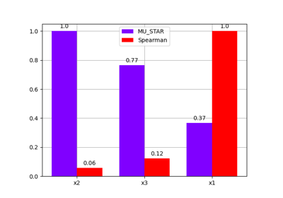
plot(output, inputs=(), title='', save=True, show=False, file_path='', directory_path='', file_name='', file_format='')[source]

Plot the sensitivity indices.

Parameters:

output (VariableType) – The output for which to display sensitivity indices, either a name or a tuple of the form (name, component). If name, its first component is considered.
inputs (Iterable[str]) –
The uncertain input variables for which to display the sensitivity indices. If empty, display all the uncertain input variables.

By default it is set to ().
title (str) –
The title of the plot, if any.

By default it is set to “”.
save (bool) –
If True, save the figure.

By default it is set to True.
show (bool) –
If True, show the figure.

By default it is set to False.
file_path (str | Path) –
A file path. Either a complete file path, a directory name or a file name. If empty, use a default file name and a default directory. The file extension is inferred from filepath extension, if any.

By default it is set to “”.
directory_path (str | Path) –
The path to the directory where to save the plots.

By default it is set to “”.
file_name (str) –
The name of the file.

By default it is set to “”.
file_format (str) –
A file format, e.g. ‘png’, ‘pdf’, ‘svg’, … Used when file_path does not have any extension. If empty, use a default file extension.

By default it is set to “”.

Returns:

The plot figure.

Return type:

RadarChart

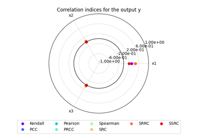
plot_radar(outputs=(), inputs=(), title='', save=True, show=False, file_path='', directory_path='', file_name='', file_format='', min_radius=-1.0, max_radius=1.0, **options)[source]

Plot the sensitivity indices on a radar chart.

This method may consider one or more outputs, as well as all inputs (default behavior) or a subset.

For visualization purposes, it is also possible to change the minimum and maximum radius values.

Parameters:

outputs (OutputsType) –
The outputs for which to display sensitivity indices, either a name, a list of names, a (name, component) tuple, a list of such tuples or a list mixing such tuples and names. When a name is specified, all its components are considered. If empty, use the default outputs.

By default it is set to ().
inputs (Iterable[str]) –
The uncertain input variables for which to display the sensitivity indices. If empty, display all the uncertain input variables.

By default it is set to ().
title (str) –
The title of the plot, if any.

By default it is set to “”.
save (bool) –
If True, save the figure.

By default it is set to True.
show (bool) –
If True, show the figure.

By default it is set to False.
file_path (str | Path) –
The path of the file to save the figures. If the extension is missing, use file_extension. If empty, create a file path from directory_path, file_name and file_extension.

By default it is set to “”.
directory_path (str | Path) –
The path of the directory to save the figures. If empty, use the current working directory.

By default it is set to “”.
file_name (str) –
The name of the file to save the figures. If empty, use a default one generated by the post-processing.

By default it is set to “”.
file_format (str) –
A file extension, e.g. ‘png’, ‘pdf’, ‘svg’, … If empty, use a default file extension.

By default it is set to “”.
min_radius (float) –
The minimal radial value. If None, from data.

By default it is set to -1.0.
max_radius (float) –
The maximal radial value. If None, from data.

By default it is set to 1.0.
**options (bool) – The options to instantiate the RadarChart.

Returns:

A radar chart representing the sensitivity indices.

Return type:

RadarChart

DEFAULT_DRIVER = 'OT_MONTE_CARLO'

dataset: IODataset: The dataset containing the discipline evaluations.

default_output: Iterable[str]: The default outputs of interest.

property kendall: dict[str, list[dict[str, ndarray]]]

The Kendall rank correlation coefficients.

With the following structure:

{
    "output_name": [
        {
            "input_name": data_array,
        }
    ]
}

property pcc: dict[str, list[dict[str, ndarray]]]

The Partial Correlation Coefficients.

With the following structure:

{
    "output_name": [
        {
            "input_name": data_array,
        }
    ]
}

property pearson: dict[str, list[dict[str, ndarray]]]

The Pearson coefficients.

With the following structure:

{
    "output_name": [
        {
            "input_name": data_array,
        }
    ]
}

property prcc: dict[str, list[dict[str, ndarray]]]

The Partial Rank Correlation Coefficients.

With the following structure:

{
    "output_name": [
        {
            "input_name": data_array,
        }
    ]
}

property spearman: dict[str, list[dict[str, ndarray]]]

The Spearman coefficients.

ith the following structure:

{
    "output_name": [
        {
            "input_name": data_array,
        }
    ]
}

property src: dict[str, list[dict[str, ndarray]]]

The Standard Regression Coefficients.

With the following structure:

{
    "output_name": [
        {
            "input_name": data_array,
        }
    ]
}

property srrc: dict[str, list[dict[str, ndarray]]]

The Standard Rank Regression Coefficients.

With the following structure:

{
    "output_name": [
        {
            "input_name": data_array,
        }
    ]
}

property ssrc: dict[str, list[dict[str, ndarray]]]

The Squared Standard Regression Coefficients.

With the following structure:

{
    "output_name": [
        {
            "input_name": data_array,
        }
    ]
}

Examples using CorrelationAnalysis¶

Comparing sensitivity indices

Correlation analysis