Note
Go to the end to download the full example code
Morris analysis
from __future__ import annotations

import pprint

from gemseo import configure_logger
from gemseo.problems.uncertainty.ishigami.ishigami_discipline import IshigamiDiscipline
from gemseo.problems.uncertainty.ishigami.ishigami_space import IshigamiSpace
from gemseo.uncertainty.sensitivity.morris.analysis import MorrisAnalysis

configure_logger()
<RootLogger root (INFO)>
In this example, we consider the Ishigami function [IH90]
implemented as an MDODiscipline by the IshigamiDiscipline.
It is commonly used
with the independent random variables \(X_1\), \(X_2\) and \(X_3\)
uniformly distributed between \(-\pi\) and \(\pi\)
and defined in the IshigamiSpace.
discipline = IshigamiDiscipline()
uncertain_space = IshigamiSpace()
Then,
we run sensitivity analysis of type MorrisAnalysis:
sensitivity_analysis = MorrisAnalysis([discipline], uncertain_space, n_samples=None)
sensitivity_analysis.compute_indices()
WARNING - 08:55:22: No coupling in MDA, switching chain_linearize to True.
WARNING - 08:55:22: No coupling in MDA, switching chain_linearize to True.
INFO - 08:55:22:
INFO - 08:55:22: *** Start MorrisAnalysisSamplingPhase execution ***
INFO - 08:55:22: MorrisAnalysisSamplingPhase
INFO - 08:55:22: Disciplines: _OATSensitivity
INFO - 08:55:22: MDO formulation: MDF
INFO - 08:55:22: Running the algorithm lhs:
INFO - 08:55:22: 20%|██ | 1/5 [00:00<00:00, 55.75 it/sec]
INFO - 08:55:22: 40%|████ | 2/5 [00:00<00:00, 90.19 it/sec]
INFO - 08:55:22: 60%|██████ | 3/5 [00:00<00:00, 114.55 it/sec]
INFO - 08:55:22: 80%|████████ | 4/5 [00:00<00:00, 132.27 it/sec]
INFO - 08:55:22: 100%|██████████| 5/5 [00:00<00:00, 146.04 it/sec]
INFO - 08:55:22: *** End MorrisAnalysisSamplingPhase execution (time: 0:00:00.046215) ***
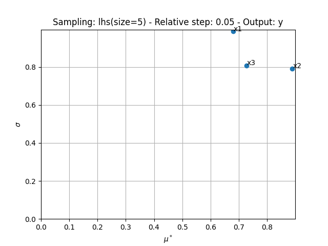
{'MU': {'y': [{'x1': array([-0.36000398]), 'x2': array([0.77781853]), 'x3': array([-0.70990541])}]}, 'MU_STAR': {'y': [{'x1': array([0.67947346]), 'x2': array([0.88906579]), 'x3': array([0.72694219])}]}, 'SIGMA': {'y': [{'x1': array([0.98724949]), 'x2': array([0.79064599]), 'x3': array([0.8074493])}]}, 'RELATIVE_SIGMA': {'y': [{'x1': array([1.45296254]), 'x2': array([0.88929976]), 'x3': array([1.11074761])}]}, 'MIN': {'y': [{'x1': array([0.0338188]), 'x2': array([0.11821721]), 'x3': array([8.72820113e-05])}]}, 'MAX': {'y': [{'x1': array([2.2360336]), 'x2': array([1.83987522]), 'x3': array([2.12052546])}]}}
The resulting indices are the empirical means and the standard deviations of the absolute output variations due to input changes.
pprint.pprint(sensitivity_analysis.indices)
{'MAX': {'y': [{'x1': array([2.2360336]),
                'x2': array([1.83987522]),
                'x3': array([2.12052546])}]},
 'MIN': {'y': [{'x1': array([0.0338188]),
                'x2': array([0.11821721]),
                'x3': array([8.72820113e-05])}]},
 'MU': {'y': [{'x1': array([-0.36000398]),
               'x2': array([0.77781853]),
               'x3': array([-0.70990541])}]},
 'MU_STAR': {'y': [{'x1': array([0.67947346]),
                    'x2': array([0.88906579]),
                    'x3': array([0.72694219])}]},
 'RELATIVE_SIGMA': {'y': [{'x1': array([1.45296254]),
                           'x2': array([0.88929976]),
                           'x3': array([1.11074761])}]},
 'SIGMA': {'y': [{'x1': array([0.98724949]),
                  'x2': array([0.79064599]),
                  'x3': array([0.8074493])}]}}
The main indices corresponds to these empirical means
(this main method can be changed with MorrisAnalysis.main_method):
pprint.pprint(sensitivity_analysis.main_indices)
{'y': [{'x1': array([0.67947346]),
        'x2': array([0.88906579]),
        'x3': array([0.72694219])}]}
and can be interpreted with respect to the empirical bounds of the outputs:
pprint.pprint(sensitivity_analysis.outputs_bounds)
{'y': [array([-1.00881748]), array([14.89344259])]}
We can also get the input parameters sorted by decreasing order of influence:
sensitivity_analysis.sort_parameters("y")
['x2', 'x3', 'x1']
We can use the method MorrisAnalysis.plot()
to visualize the different series of indices:
sensitivity_analysis.plot("y", save=False, show=True, lower_mu=0, lower_sigma=0)
<Figure size 640x480 with 1 Axes>
Lastly,
the sensitivity indices can be exported to a Dataset:
sensitivity_analysis.to_dataset()
Total running time of the script: (0 minutes 0.462 seconds)