Note
Go to the end to download the full example code.
Linear regression#
A LinearRegressor is a linear regression model
based on scikit-learn.
See also
You can find more information about building linear models with scikit-learn on this page.
from __future__ import annotations

from matplotlib import pyplot as plt
from numpy import array

from gemseo import create_design_space
from gemseo import create_discipline
from gemseo import sample_disciplines
from gemseo.mlearning import create_regression_model
Problem#
In this example,
we represent the function \(f(x)=(6x-2)^2\sin(12x-4)\) [FSK08]
by the AnalyticDiscipline
discipline = create_discipline(
    "AnalyticDiscipline",
    name="f",
    expressions={"y": "(6*x-2)**2*sin(12*x-4)"},
)
and seek to approximate it over the input space
input_space = create_design_space()
input_space.add_variable("x", lower_bound=0.0, upper_bound=1.0)
To do this, we create a training dataset with 6 equispaced points:
training_dataset = sample_disciplines(
    [discipline], input_space, "y", algo_name="PYDOE_FULLFACT", n_samples=6
)
INFO - 16:16:09: *** Start Sampling execution ***
INFO - 16:16:09: Sampling
INFO - 16:16:09:    Disciplines: f
INFO - 16:16:09:    MDO formulation: MDF
INFO - 16:16:09: Running the algorithm PYDOE_FULLFACT:
INFO - 16:16:09:     17%|█▋        | 1/6 [00:00<00:00, 649.68 it/sec]
INFO - 16:16:09:     33%|███▎      | 2/6 [00:00<00:00, 1054.51 it/sec]
INFO - 16:16:09:     50%|█████     | 3/6 [00:00<00:00, 1386.70 it/sec]
INFO - 16:16:09:     67%|██████▋   | 4/6 [00:00<00:00, 1660.78 it/sec]
INFO - 16:16:09:     83%|████████▎ | 5/6 [00:00<00:00, 1896.50 it/sec]
INFO - 16:16:09:    100%|██████████| 6/6 [00:00<00:00, 2030.48 it/sec]
INFO - 16:16:09: *** End Sampling execution ***
Basics#
Training#
Then, we train a linear regression model from these samples:
model = create_regression_model("LinearRegressor", training_dataset)
model.learn()
Prediction#
Once it is built, we can predict the output value of \(f\) at a new input point:
input_value = {"x": array([0.65])}
output_value = model.predict(input_value)
output_value
{'y': array([3.29457456])}
as well as its Jacobian value:
jacobian_value = model.predict_jacobian(input_value)
jacobian_value
{'y': {'x': array([[7.26002643]])}}
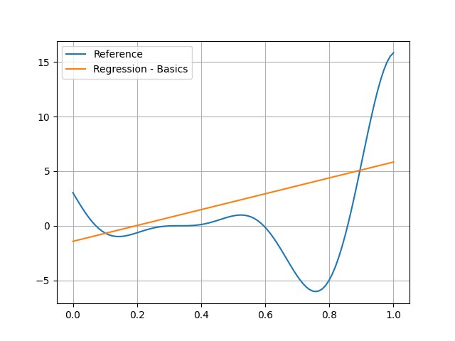
Plotting#
Of course, you can see that the linear model is no good at all here:
test_dataset = sample_disciplines(
    [discipline], input_space, "y", algo_name="PYDOE_FULLFACT", n_samples=100
)
input_data = test_dataset.get_view(variable_names=model.input_names).to_numpy()
reference_output_data = test_dataset.get_view(variable_names="y").to_numpy().ravel()
predicted_output_data = model.predict(input_data).ravel()
plt.plot(input_data.ravel(), reference_output_data, label="Reference")
plt.plot(input_data.ravel(), predicted_output_data, label="Regression - Basics")
plt.grid()
plt.legend()
plt.show()
INFO - 16:16:09: *** Start Sampling execution ***
INFO - 16:16:09: Sampling
INFO - 16:16:09:    Disciplines: f
INFO - 16:16:09:    MDO formulation: MDF
INFO - 16:16:09: Running the algorithm PYDOE_FULLFACT:
INFO - 16:16:09:      1%|          | 1/100 [00:00<00:00, 3990.77 it/sec]
INFO - 16:16:09:      2%|▏         | 2/100 [00:00<00:00, 3788.89 it/sec]
INFO - 16:16:09:      3%|▎         | 3/100 [00:00<00:00, 3888.42 it/sec]
INFO - 16:16:09:      4%|▍         | 4/100 [00:00<00:00, 3982.25 it/sec]
INFO - 16:16:09:      5%|▌         | 5/100 [00:00<00:00, 3950.93 it/sec]
INFO - 16:16:09:      6%|▌         | 6/100 [00:00<00:00, 4016.89 it/sec]
INFO - 16:16:09:      7%|▋         | 7/100 [00:00<00:00, 4077.23 it/sec]
INFO - 16:16:09:      8%|▊         | 8/100 [00:00<00:00, 4130.79 it/sec]
INFO - 16:16:09:      9%|▉         | 9/100 [00:00<00:00, 4129.61 it/sec]
INFO - 16:16:09:     10%|█         | 10/100 [00:00<00:00, 4161.43 it/sec]
INFO - 16:16:09:     11%|█         | 11/100 [00:00<00:00, 4187.83 it/sec]
INFO - 16:16:09:     12%|█▏        | 12/100 [00:00<00:00, 4222.45 it/sec]
INFO - 16:16:09:     13%|█▎        | 13/100 [00:00<00:00, 4246.90 it/sec]
INFO - 16:16:09:     14%|█▍        | 14/100 [00:00<00:00, 4237.59 it/sec]
INFO - 16:16:09:     15%|█▌        | 15/100 [00:00<00:00, 4267.42 it/sec]
INFO - 16:16:09:     16%|█▌        | 16/100 [00:00<00:00, 4296.62 it/sec]
INFO - 16:16:09:     17%|█▋        | 17/100 [00:00<00:00, 4316.17 it/sec]
INFO - 16:16:09:     18%|█▊        | 18/100 [00:00<00:00, 4314.39 it/sec]
INFO - 16:16:09:     19%|█▉        | 19/100 [00:00<00:00, 4328.25 it/sec]
INFO - 16:16:09:     20%|██        | 20/100 [00:00<00:00, 4347.78 it/sec]
INFO - 16:16:09:     21%|██        | 21/100 [00:00<00:00, 4360.63 it/sec]
INFO - 16:16:09:     22%|██▏       | 22/100 [00:00<00:00, 4372.79 it/sec]
INFO - 16:16:09:     23%|██▎       | 23/100 [00:00<00:00, 4365.90 it/sec]
INFO - 16:16:09:     24%|██▍       | 24/100 [00:00<00:00, 4377.81 it/sec]
INFO - 16:16:09:     25%|██▌       | 25/100 [00:00<00:00, 4392.31 it/sec]
INFO - 16:16:09:     26%|██▌       | 26/100 [00:00<00:00, 4404.18 it/sec]
INFO - 16:16:09:     27%|██▋       | 27/100 [00:00<00:00, 4400.65 it/sec]
INFO - 16:16:09:     28%|██▊       | 28/100 [00:00<00:00, 4404.96 it/sec]
INFO - 16:16:09:     29%|██▉       | 29/100 [00:00<00:00, 4405.30 it/sec]
INFO - 16:16:09:     30%|███       | 30/100 [00:00<00:00, 4415.21 it/sec]
INFO - 16:16:09:     31%|███       | 31/100 [00:00<00:00, 4426.03 it/sec]
INFO - 16:16:09:     32%|███▏      | 32/100 [00:00<00:00, 4370.63 it/sec]
INFO - 16:16:09:     33%|███▎      | 33/100 [00:00<00:00, 4374.04 it/sec]
INFO - 16:16:09:     34%|███▍      | 34/100 [00:00<00:00, 4384.65 it/sec]
INFO - 16:16:09:     35%|███▌      | 35/100 [00:00<00:00, 4394.57 it/sec]
INFO - 16:16:09:     36%|███▌      | 36/100 [00:00<00:00, 4388.88 it/sec]
INFO - 16:16:09:     37%|███▋      | 37/100 [00:00<00:00, 4394.18 it/sec]
INFO - 16:16:09:     38%|███▊      | 38/100 [00:00<00:00, 4403.71 it/sec]
INFO - 16:16:09:     39%|███▉      | 39/100 [00:00<00:00, 4413.03 it/sec]
INFO - 16:16:09:     40%|████      | 40/100 [00:00<00:00, 4421.46 it/sec]
INFO - 16:16:09:     41%|████      | 41/100 [00:00<00:00, 4415.85 it/sec]
INFO - 16:16:09:     42%|████▏     | 42/100 [00:00<00:00, 4422.93 it/sec]
INFO - 16:16:09:     43%|████▎     | 43/100 [00:00<00:00, 4429.80 it/sec]
INFO - 16:16:09:     44%|████▍     | 44/100 [00:00<00:00, 4436.28 it/sec]
INFO - 16:16:09:     45%|████▌     | 45/100 [00:00<00:00, 4433.00 it/sec]
INFO - 16:16:09:     46%|████▌     | 46/100 [00:00<00:00, 4436.27 it/sec]
INFO - 16:16:09:     47%|████▋     | 47/100 [00:00<00:00, 4438.92 it/sec]
INFO - 16:16:09:     48%|████▊     | 48/100 [00:00<00:00, 4443.31 it/sec]
INFO - 16:16:09:     49%|████▉     | 49/100 [00:00<00:00, 4448.89 it/sec]
INFO - 16:16:09:     50%|█████     | 50/100 [00:00<00:00, 4443.68 it/sec]
INFO - 16:16:09:     51%|█████     | 51/100 [00:00<00:00, 4446.26 it/sec]
INFO - 16:16:09:     52%|█████▏    | 52/100 [00:00<00:00, 4449.46 it/sec]
INFO - 16:16:09:     53%|█████▎    | 53/100 [00:00<00:00, 4450.95 it/sec]
INFO - 16:16:09:     54%|█████▍    | 54/100 [00:00<00:00, 4447.31 it/sec]
INFO - 16:16:09:     55%|█████▌    | 55/100 [00:00<00:00, 4448.34 it/sec]
INFO - 16:16:09:     56%|█████▌    | 56/100 [00:00<00:00, 4450.78 it/sec]
INFO - 16:16:09:     57%|█████▋    | 57/100 [00:00<00:00, 4453.38 it/sec]
INFO - 16:16:09:     58%|█████▊    | 58/100 [00:00<00:00, 4457.69 it/sec]
INFO - 16:16:09:     59%|█████▉    | 59/100 [00:00<00:00, 4450.95 it/sec]
INFO - 16:16:09:     60%|██████    | 60/100 [00:00<00:00, 4453.42 it/sec]
INFO - 16:16:09:     61%|██████    | 61/100 [00:00<00:00, 4421.92 it/sec]
INFO - 16:16:09:     62%|██████▏   | 62/100 [00:00<00:00, 4422.79 it/sec]
INFO - 16:16:09:     63%|██████▎   | 63/100 [00:00<00:00, 4417.71 it/sec]
INFO - 16:16:09:     64%|██████▍   | 64/100 [00:00<00:00, 4419.85 it/sec]
INFO - 16:16:09:     65%|██████▌   | 65/100 [00:00<00:00, 4419.14 it/sec]
INFO - 16:16:09:     66%|██████▌   | 66/100 [00:00<00:00, 4423.17 it/sec]
INFO - 16:16:09:     67%|██████▋   | 67/100 [00:00<00:00, 4421.80 it/sec]
INFO - 16:16:09:     68%|██████▊   | 68/100 [00:00<00:00, 4424.78 it/sec]
INFO - 16:16:09:     69%|██████▉   | 69/100 [00:00<00:00, 4411.09 it/sec]
INFO - 16:16:09:     70%|███████   | 70/100 [00:00<00:00, 4411.08 it/sec]
INFO - 16:16:09:     71%|███████   | 71/100 [00:00<00:00, 4409.30 it/sec]
INFO - 16:16:09:     72%|███████▏  | 72/100 [00:00<00:00, 4410.87 it/sec]
INFO - 16:16:09:     73%|███████▎  | 73/100 [00:00<00:00, 4413.59 it/sec]
INFO - 16:16:09:     74%|███████▍  | 74/100 [00:00<00:00, 4416.75 it/sec]
INFO - 16:16:09:     75%|███████▌  | 75/100 [00:00<00:00, 4420.58 it/sec]
INFO - 16:16:09:     76%|███████▌  | 76/100 [00:00<00:00, 4419.10 it/sec]
INFO - 16:16:09:     77%|███████▋  | 77/100 [00:00<00:00, 4421.28 it/sec]
INFO - 16:16:09:     78%|███████▊  | 78/100 [00:00<00:00, 4424.13 it/sec]
INFO - 16:16:09:     79%|███████▉  | 79/100 [00:00<00:00, 4426.26 it/sec]
INFO - 16:16:09:     80%|████████  | 80/100 [00:00<00:00, 4425.19 it/sec]
INFO - 16:16:09:     81%|████████  | 81/100 [00:00<00:00, 4426.50 it/sec]
INFO - 16:16:09:     82%|████████▏ | 82/100 [00:00<00:00, 4429.21 it/sec]
INFO - 16:16:09:     83%|████████▎ | 83/100 [00:00<00:00, 4427.07 it/sec]
INFO - 16:16:09:     84%|████████▍ | 84/100 [00:00<00:00, 4430.60 it/sec]
INFO - 16:16:09:     85%|████████▌ | 85/100 [00:00<00:00, 4428.77 it/sec]
INFO - 16:16:09:     86%|████████▌ | 86/100 [00:00<00:00, 4430.29 it/sec]
INFO - 16:16:09:     87%|████████▋ | 87/100 [00:00<00:00, 4432.32 it/sec]
INFO - 16:16:09:     88%|████████▊ | 88/100 [00:00<00:00, 4434.63 it/sec]
INFO - 16:16:09:     89%|████████▉ | 89/100 [00:00<00:00, 4438.05 it/sec]
INFO - 16:16:09:     90%|█████████ | 90/100 [00:00<00:00, 4434.61 it/sec]
INFO - 16:16:09:     91%|█████████ | 91/100 [00:00<00:00, 4437.02 it/sec]
INFO - 16:16:09:     92%|█████████▏| 92/100 [00:00<00:00, 4440.15 it/sec]
INFO - 16:16:09:     93%|█████████▎| 93/100 [00:00<00:00, 4443.47 it/sec]
INFO - 16:16:09:     94%|█████████▍| 94/100 [00:00<00:00, 4442.67 it/sec]
INFO - 16:16:09:     95%|█████████▌| 95/100 [00:00<00:00, 4444.16 it/sec]
INFO - 16:16:09:     96%|█████████▌| 96/100 [00:00<00:00, 4447.14 it/sec]
INFO - 16:16:09:     97%|█████████▋| 97/100 [00:00<00:00, 4450.12 it/sec]
INFO - 16:16:09:     98%|█████████▊| 98/100 [00:00<00:00, 4454.34 it/sec]
INFO - 16:16:09:     99%|█████████▉| 99/100 [00:00<00:00, 4453.13 it/sec]
INFO - 16:16:09:    100%|██████████| 100/100 [00:00<00:00, 4397.37 it/sec]
INFO - 16:16:09: *** End Sampling execution ***
Settings#
The LinearRegressor has many options
defined in the LinearRegressor_Settings Pydantic model.
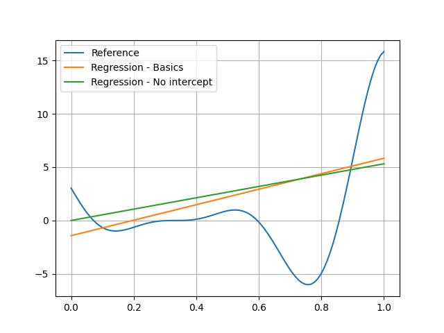
Intercept#
By default,
the linear model is of the form \(a_0+a_1x_1+\ldots+a_dx_d\).
You can set the option fit_intercept to False
if you want a linear model of the form \(a_1x_1+\ldots+a_dx_d\):
model = create_regression_model(
    "LinearRegressor", training_dataset, fit_intercept=False, transformer={}
)
model.learn()
Warning
This notion applies in the space of transformed variables.
This is the reason why
we removed the default transformers by setting transformer to {}.
We can see the impact of this option in the following visualization:
predicted_output_data_ = model.predict(input_data).ravel()
plt.plot(input_data.ravel(), reference_output_data, label="Reference")
plt.plot(input_data.ravel(), predicted_output_data, label="Regression - Basics")
plt.plot(input_data.ravel(), predicted_output_data_, label="Regression - No intercept")
plt.grid()
plt.legend()
plt.show()
Regularization#
When the number of samples is small relative to the input dimension,
regularization techniques can save you from overfitting
(a model that is very good at learning but bad at generalization).
The penalty_level option is a positive real number
defining the degree of regularization (default: no regularization).
By default,
the regularization technique is the ridge penalty (l2 regularization).
The technique can be replaced by the lasso penalty (l1 regularization)
by setting the l2_penalty_ratio option to 0.0.
When l2_penalty_ratio is between 0 and 1,
the regularization technique is the elastic net penalty,
i.e. a linear combination of ridge and lasso penalty
parametrized by this l2_penalty_ratio.
For example, we can use the ridge penalty with a level of 1.2
model = create_regression_model("LinearRegressor", training_dataset, penalty_level=1.2)
model.learn()
predicted_output_data_ = model.predict(input_data).ravel()
plt.plot(input_data.ravel(), reference_output_data, label="Reference")
plt.plot(input_data.ravel(), predicted_output_data, label="Regression - Basics")
plt.plot(input_data.ravel(), predicted_output_data_, label="Regression - Ridge(1.2)")
plt.grid()
plt.legend()
plt.show()
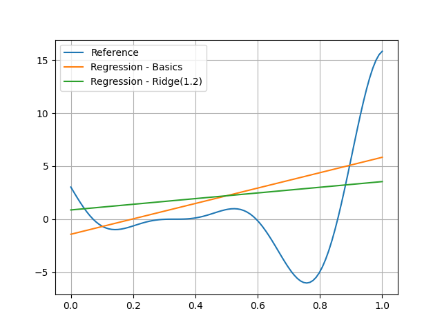
We can see that the coefficient of the linear model is lower due to the penalty.
Note
In the case of a model with many inputs, we could have used the lasso penalty and seen that some coefficients would have been set to zero.
Total running time of the script: (0 minutes 0.192 seconds)