Note
Go to the end to download the full example code.
Radial basis function (RBF) regression#
An RBFRegressor is an RBF model
based on SciPy.
See also
You can find more information about RBF models on this wikipedia page.
from __future__ import annotations

from matplotlib import pyplot as plt
from numpy import array

from gemseo import create_design_space
from gemseo import create_discipline
from gemseo import sample_disciplines
from gemseo.mlearning import create_regression_model
from gemseo.mlearning.regression.algos.rbf_settings import RBF
Problem#
In this example,
we represent the function \(f(x)=(6x-2)^2\sin(12x-4)\) [FSK08]
by the AnalyticDiscipline
discipline = create_discipline(
    "AnalyticDiscipline",
    name="f",
    expressions={"y": "(6*x-2)**2*sin(12*x-4)"},
)
and seek to approximate it over the input space
input_space = create_design_space()
input_space.add_variable("x", lower_bound=0.0, upper_bound=1.0)
To do this, we create a training dataset with 6 equispaced points:
training_dataset = sample_disciplines(
    [discipline], input_space, "y", algo_name="PYDOE_FULLFACT", n_samples=6
)
INFO - 16:16:12: *** Start Sampling execution ***
INFO - 16:16:12: Sampling
INFO - 16:16:12:    Disciplines: f
INFO - 16:16:12:    MDO formulation: MDF
INFO - 16:16:12: Running the algorithm PYDOE_FULLFACT:
INFO - 16:16:12:     17%|█▋        | 1/6 [00:00<00:00, 667.25 it/sec]
INFO - 16:16:12:     33%|███▎      | 2/6 [00:00<00:00, 1071.89 it/sec]
INFO - 16:16:12:     50%|█████     | 3/6 [00:00<00:00, 1409.06 it/sec]
INFO - 16:16:12:     67%|██████▋   | 4/6 [00:00<00:00, 1630.44 it/sec]
INFO - 16:16:12:     83%|████████▎ | 5/6 [00:00<00:00, 1855.56 it/sec]
INFO - 16:16:12:    100%|██████████| 6/6 [00:00<00:00, 1978.29 it/sec]
INFO - 16:16:12: *** End Sampling execution ***
Basics#
Training#
Then, we train an RBF regression model from these samples:
model = create_regression_model("RBFRegressor", training_dataset)
model.learn()
Prediction#
Once it is built, we can predict the output value of \(f\) at a new input point:
input_value = {"x": array([0.65])}
output_value = model.predict(input_value)
output_value
{'y': array([-2.16802353])}
as well as its Jacobian value:
jacobian_value = model.predict_jacobian(input_value)
jacobian_value
{'y': {'x': array([[-45.81825011]])}}
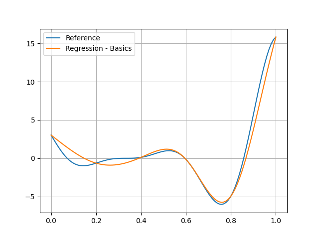
Plotting#
You can see that the RBF model is pretty good on the right, but bad on the left:
test_dataset = sample_disciplines(
    [discipline], input_space, "y", algo_name="PYDOE_FULLFACT", n_samples=100
)
input_data = test_dataset.get_view(variable_names=model.input_names).to_numpy()
reference_output_data = test_dataset.get_view(variable_names="y").to_numpy().ravel()
predicted_output_data = model.predict(input_data).ravel()
plt.plot(input_data.ravel(), reference_output_data, label="Reference")
plt.plot(input_data.ravel(), predicted_output_data, label="Regression - Basics")
plt.grid()
plt.legend()
plt.show()
INFO - 16:16:12: *** Start Sampling execution ***
INFO - 16:16:12: Sampling
INFO - 16:16:12:    Disciplines: f
INFO - 16:16:12:    MDO formulation: MDF
INFO - 16:16:12: Running the algorithm PYDOE_FULLFACT:
INFO - 16:16:12:      1%|          | 1/100 [00:00<00:00, 3986.98 it/sec]
INFO - 16:16:12:      2%|▏         | 2/100 [00:00<00:00, 3775.25 it/sec]
INFO - 16:16:12:      3%|▎         | 3/100 [00:00<00:00, 3825.76 it/sec]
INFO - 16:16:12:      4%|▍         | 4/100 [00:00<00:00, 3927.25 it/sec]
INFO - 16:16:12:      5%|▌         | 5/100 [00:00<00:00, 3922.11 it/sec]
INFO - 16:16:12:      6%|▌         | 6/100 [00:00<00:00, 3989.51 it/sec]
INFO - 16:16:12:      7%|▋         | 7/100 [00:00<00:00, 4051.35 it/sec]
INFO - 16:16:12:      8%|▊         | 8/100 [00:00<00:00, 4113.58 it/sec]
INFO - 16:16:12:      9%|▉         | 9/100 [00:00<00:00, 4161.02 it/sec]
INFO - 16:16:12:     10%|█         | 10/100 [00:00<00:00, 4148.26 it/sec]
INFO - 16:16:12:     11%|█         | 11/100 [00:00<00:00, 4185.17 it/sec]
INFO - 16:16:12:     12%|█▏        | 12/100 [00:00<00:00, 4222.45 it/sec]
INFO - 16:16:12:     13%|█▎        | 13/100 [00:00<00:00, 4249.55 it/sec]
INFO - 16:16:12:     14%|█▍        | 14/100 [00:00<00:00, 4245.25 it/sec]
INFO - 16:16:12:     15%|█▌        | 15/100 [00:00<00:00, 4268.00 it/sec]
INFO - 16:16:12:     16%|█▌        | 16/100 [00:00<00:00, 4289.48 it/sec]
INFO - 16:16:12:     17%|█▋        | 17/100 [00:00<00:00, 4312.26 it/sec]
INFO - 16:16:12:     18%|█▊        | 18/100 [00:00<00:00, 4336.19 it/sec]
INFO - 16:16:12:     19%|█▉        | 19/100 [00:00<00:00, 4328.02 it/sec]
INFO - 16:16:12:     20%|██        | 20/100 [00:00<00:00, 4346.88 it/sec]
INFO - 16:16:12:     21%|██        | 21/100 [00:00<00:00, 4352.87 it/sec]
INFO - 16:16:12:     22%|██▏       | 22/100 [00:00<00:00, 4367.83 it/sec]
INFO - 16:16:12:     23%|██▎       | 23/100 [00:00<00:00, 4365.51 it/sec]
INFO - 16:16:12:     24%|██▍       | 24/100 [00:00<00:00, 4376.28 it/sec]
INFO - 16:16:12:     25%|██▌       | 25/100 [00:00<00:00, 4389.18 it/sec]
INFO - 16:16:12:     26%|██▌       | 26/100 [00:00<00:00, 4400.45 it/sec]
INFO - 16:16:12:     27%|██▋       | 27/100 [00:00<00:00, 4411.45 it/sec]
INFO - 16:16:12:     28%|██▊       | 28/100 [00:00<00:00, 4401.16 it/sec]
INFO - 16:16:12:     29%|██▉       | 29/100 [00:00<00:00, 4405.62 it/sec]
INFO - 16:16:12:     30%|███       | 30/100 [00:00<00:00, 4414.75 it/sec]
INFO - 16:16:12:     31%|███       | 31/100 [00:00<00:00, 4423.77 it/sec]
INFO - 16:16:12:     32%|███▏      | 32/100 [00:00<00:00, 4421.60 it/sec]
INFO - 16:16:12:     33%|███▎      | 33/100 [00:00<00:00, 4428.48 it/sec]
INFO - 16:16:12:     34%|███▍      | 34/100 [00:00<00:00, 4438.56 it/sec]
INFO - 16:16:12:     35%|███▌      | 35/100 [00:00<00:00, 4448.37 it/sec]
INFO - 16:16:12:     36%|███▌      | 36/100 [00:00<00:00, 4456.49 it/sec]
INFO - 16:16:12:     37%|███▋      | 37/100 [00:00<00:00, 4451.91 it/sec]
INFO - 16:16:12:     38%|███▊      | 38/100 [00:00<00:00, 4458.28 it/sec]
INFO - 16:16:12:     39%|███▉      | 39/100 [00:00<00:00, 4463.00 it/sec]
INFO - 16:16:12:     40%|████      | 40/100 [00:00<00:00, 4471.30 it/sec]
INFO - 16:16:12:     41%|████      | 41/100 [00:00<00:00, 4479.23 it/sec]
INFO - 16:16:12:     42%|████▏     | 42/100 [00:00<00:00, 4474.27 it/sec]
INFO - 16:16:12:     43%|████▎     | 43/100 [00:00<00:00, 4480.87 it/sec]
INFO - 16:16:12:     44%|████▍     | 44/100 [00:00<00:00, 4488.07 it/sec]
INFO - 16:16:12:     45%|████▌     | 45/100 [00:00<00:00, 4491.87 it/sec]
INFO - 16:16:12:     46%|████▌     | 46/100 [00:00<00:00, 4488.29 it/sec]
INFO - 16:16:12:     47%|████▋     | 47/100 [00:00<00:00, 4492.94 it/sec]
INFO - 16:16:12:     48%|████▊     | 48/100 [00:00<00:00, 4498.32 it/sec]
INFO - 16:16:12:     49%|████▉     | 49/100 [00:00<00:00, 4499.14 it/sec]
INFO - 16:16:12:     50%|█████     | 50/100 [00:00<00:00, 4504.19 it/sec]
INFO - 16:16:12:     51%|█████     | 51/100 [00:00<00:00, 4497.20 it/sec]
INFO - 16:16:12:     52%|█████▏    | 52/100 [00:00<00:00, 4501.25 it/sec]
INFO - 16:16:12:     53%|█████▎    | 53/100 [00:00<00:00, 4506.26 it/sec]
INFO - 16:16:12:     54%|█████▍    | 54/100 [00:00<00:00, 4511.26 it/sec]
INFO - 16:16:12:     55%|█████▌    | 55/100 [00:00<00:00, 4507.54 it/sec]
INFO - 16:16:12:     56%|█████▌    | 56/100 [00:00<00:00, 4509.57 it/sec]
INFO - 16:16:12:     57%|█████▋    | 57/100 [00:00<00:00, 4513.84 it/sec]
INFO - 16:16:12:     58%|█████▊    | 58/100 [00:00<00:00, 4512.51 it/sec]
INFO - 16:16:12:     59%|█████▉    | 59/100 [00:00<00:00, 4517.08 it/sec]
INFO - 16:16:12:     60%|██████    | 60/100 [00:00<00:00, 4513.40 it/sec]
INFO - 16:16:12:     61%|██████    | 61/100 [00:00<00:00, 4486.28 it/sec]
INFO - 16:16:12:     62%|██████▏   | 62/100 [00:00<00:00, 4487.67 it/sec]
INFO - 16:16:12:     63%|██████▎   | 63/100 [00:00<00:00, 4491.53 it/sec]
INFO - 16:16:12:     64%|██████▍   | 64/100 [00:00<00:00, 4489.64 it/sec]
INFO - 16:16:12:     65%|██████▌   | 65/100 [00:00<00:00, 4492.24 it/sec]
INFO - 16:16:12:     66%|██████▌   | 66/100 [00:00<00:00, 4495.58 it/sec]
INFO - 16:16:12:     67%|██████▋   | 67/100 [00:00<00:00, 4497.73 it/sec]
INFO - 16:16:12:     68%|██████▊   | 68/100 [00:00<00:00, 4499.69 it/sec]
INFO - 16:16:12:     69%|██████▉   | 69/100 [00:00<00:00, 4494.80 it/sec]
INFO - 16:16:12:     70%|███████   | 70/100 [00:00<00:00, 4497.78 it/sec]
INFO - 16:16:12:     71%|███████   | 71/100 [00:00<00:00, 4501.69 it/sec]
INFO - 16:16:12:     72%|███████▏  | 72/100 [00:00<00:00, 4505.83 it/sec]
INFO - 16:16:12:     73%|███████▎  | 73/100 [00:00<00:00, 4503.44 it/sec]
INFO - 16:16:12:     74%|███████▍  | 74/100 [00:00<00:00, 4503.40 it/sec]
INFO - 16:16:12:     75%|███████▌  | 75/100 [00:00<00:00, 4504.06 it/sec]
INFO - 16:16:12:     76%|███████▌  | 76/100 [00:00<00:00, 4505.86 it/sec]
INFO - 16:16:12:     77%|███████▋  | 77/100 [00:00<00:00, 4509.19 it/sec]
INFO - 16:16:12:     78%|███████▊  | 78/100 [00:00<00:00, 4505.97 it/sec]
INFO - 16:16:12:     79%|███████▉  | 79/100 [00:00<00:00, 4507.98 it/sec]
INFO - 16:16:12:     80%|████████  | 80/100 [00:00<00:00, 4511.52 it/sec]
INFO - 16:16:12:     81%|████████  | 81/100 [00:00<00:00, 4513.72 it/sec]
INFO - 16:16:12:     82%|████████▏ | 82/100 [00:00<00:00, 4516.64 it/sec]
INFO - 16:16:12:     83%|████████▎ | 83/100 [00:00<00:00, 4512.64 it/sec]
INFO - 16:16:12:     84%|████████▍ | 84/100 [00:00<00:00, 4514.86 it/sec]
INFO - 16:16:12:     85%|████████▌ | 85/100 [00:00<00:00, 4516.23 it/sec]
INFO - 16:16:12:     86%|████████▌ | 86/100 [00:00<00:00, 4517.69 it/sec]
INFO - 16:16:12:     87%|████████▋ | 87/100 [00:00<00:00, 4513.85 it/sec]
INFO - 16:16:12:     88%|████████▊ | 88/100 [00:00<00:00, 4515.36 it/sec]
INFO - 16:16:12:     89%|████████▉ | 89/100 [00:00<00:00, 4518.14 it/sec]
INFO - 16:16:12:     90%|█████████ | 90/100 [00:00<00:00, 4520.91 it/sec]
INFO - 16:16:12:     91%|█████████ | 91/100 [00:00<00:00, 4523.15 it/sec]
INFO - 16:16:12:     92%|█████████▏| 92/100 [00:00<00:00, 4519.99 it/sec]
INFO - 16:16:12:     93%|█████████▎| 93/100 [00:00<00:00, 4522.45 it/sec]
INFO - 16:16:12:     94%|█████████▍| 94/100 [00:00<00:00, 4521.54 it/sec]
INFO - 16:16:12:     95%|█████████▌| 95/100 [00:00<00:00, 4523.73 it/sec]
INFO - 16:16:12:     96%|█████████▌| 96/100 [00:00<00:00, 4522.47 it/sec]
INFO - 16:16:12:     97%|█████████▋| 97/100 [00:00<00:00, 4523.79 it/sec]
INFO - 16:16:12:     98%|█████████▊| 98/100 [00:00<00:00, 4525.60 it/sec]
INFO - 16:16:12:     99%|█████████▉| 99/100 [00:00<00:00, 4527.46 it/sec]
INFO - 16:16:12:    100%|██████████| 100/100 [00:00<00:00, 4474.88 it/sec]
INFO - 16:16:12: *** End Sampling execution ***
Settings#
The RBFRegressor has many options
defined in the RBFRegressor_Settings Pydantic model.
Function#
The default RBF is the multiquadratic function \(\sqrt{(r/\epsilon)^2 + 1}\)
depending on a radius \(r\) representing a distance between two points
and an adjustable constant \(\epsilon\).
The RBF can be changed using the function option,
which can be either an RBF:
model = create_regression_model("RBFRegressor", training_dataset, function=RBF.GAUSSIAN)
model.learn()
predicted_output_data_g = model.predict(input_data).ravel()
or a Python function:
def rbf(self, r: float) -> float:
    """Evaluate a cubic RBF.

    An RBF must take 2 arguments, namely ``(self, r)``.

    Args:
        r: The radius.

    Returns:
        The RBF value.
    """
    return r**3


model = create_regression_model("RBFRegressor", training_dataset, function=rbf)
model.learn()
predicted_output_data_c = model.predict(input_data).ravel()
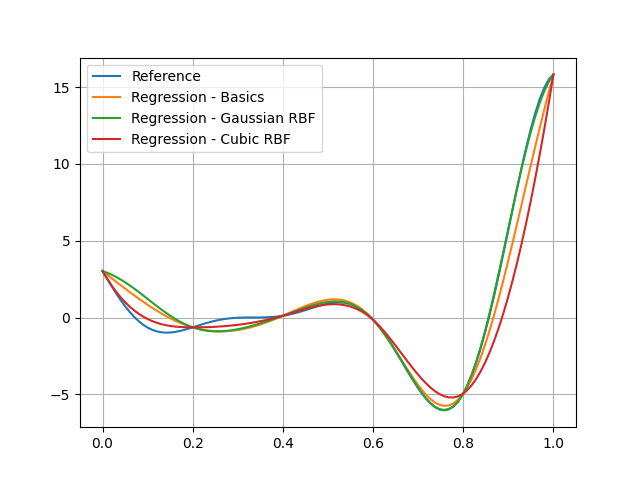
We can see that the predictions are different:
plt.plot(input_data.ravel(), reference_output_data, label="Reference")
plt.plot(input_data.ravel(), predicted_output_data, label="Regression - Basics")
plt.plot(input_data.ravel(), predicted_output_data_g, label="Regression - Gaussian RBF")
plt.plot(input_data.ravel(), predicted_output_data_c, label="Regression - Cubic RBF")
plt.grid()
plt.legend()
plt.show()
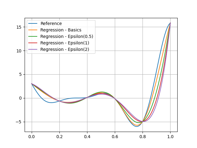
Epsilon#
Some RBFs depend on an epsilon parameter
whose default value is the average distance between input data.
This is the case of "multiquadric", "gaussian" and "inverse" RBFs.
For example,
we can train a first multiquadric RBF model with an epsilon set to 0.5
model = create_regression_model("RBFRegressor", training_dataset, epsilon=0.5)
model.learn()
predicted_output_data_1 = model.predict(input_data).ravel()
a second one with an epsilon set to 1.0:
model = create_regression_model("RBFRegressor", training_dataset, epsilon=1.0)
model.learn()
predicted_output_data_2 = model.predict(input_data).ravel()
and a last one with an epsilon set to 2.0:
model = create_regression_model("RBFRegressor", training_dataset, epsilon=2.0)
model.learn()
predicted_output_data_3 = model.predict(input_data).ravel()
and see that this parameter represents the regularity of the regression model:
plt.plot(input_data.ravel(), reference_output_data, label="Reference")
plt.plot(input_data.ravel(), predicted_output_data, label="Regression - Basics")
plt.plot(input_data.ravel(), predicted_output_data_1, label="Regression - Epsilon(0.5)")
plt.plot(input_data.ravel(), predicted_output_data_2, label="Regression - Epsilon(1)")
plt.plot(input_data.ravel(), predicted_output_data_3, label="Regression - Epsilon(2)")
plt.grid()
plt.legend()
plt.show()
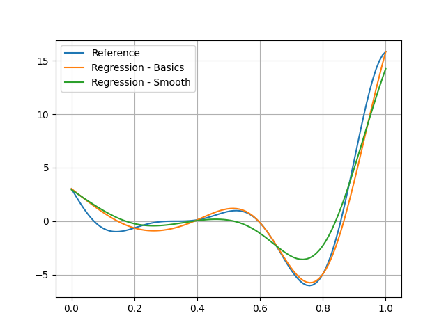
Smooth#
By default,
an RBF model interpolates the training points.
This is parametrized by the smooth option which is set to 0.
We can increase the smoothness of the model by increasing this value:
model = create_regression_model("RBFRegressor", training_dataset, smooth=0.1)
model.learn()
predicted_output_data_ = model.predict(input_data).ravel()
and see that the model is not interpolating:
plt.plot(input_data.ravel(), reference_output_data, label="Reference")
plt.plot(input_data.ravel(), predicted_output_data, label="Regression - Basics")
plt.plot(input_data.ravel(), predicted_output_data_, label="Regression - Smooth")
plt.grid()
plt.legend()
plt.show()
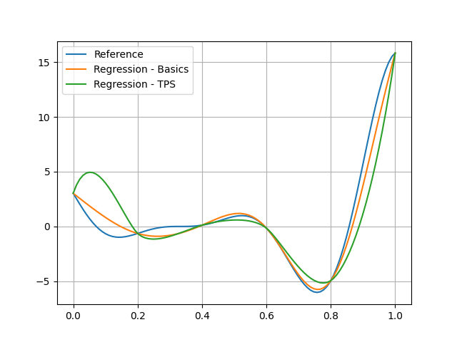
Thin plate spline (TPS)#
TPS regression is a specific case of RBF regression
where the RBF is the thin plate radial basis function for \(r^2\log(r)\).
The TPSRegressor class
deriving from RBFRegressor
implements this case:
model = create_regression_model("TPSRegressor", training_dataset)
model.learn()
predicted_output_data_ = model.predict(input_data).ravel()
We can see that the difference between this model and the default multiquadric RBF model:
plt.plot(input_data.ravel(), reference_output_data, label="Reference")
plt.plot(input_data.ravel(), predicted_output_data, label="Regression - Basics")
plt.plot(input_data.ravel(), predicted_output_data_, label="Regression - TPS")
plt.grid()
plt.legend()
plt.show()
The TPSRegressor can be customized with the TPSRegressor_Settings.
Total running time of the script: (0 minutes 0.311 seconds)