Note
Go to the end to download the full example code.
Polynomial regression#
A PolynomialRegressor is a polynomial regression model
based on a LinearRegressor.
This design choice was made
because a polynomial regression model is a generalized linear model
whose basis functions are monomials.
Thus,
a PolynomialRegressor benefits
from the same settings as LinearRegressor:
offset can be set to zero and regularization techniques can be used.
See also
You will find more information about these settings in the example about the linear regression model.
from __future__ import annotations

from matplotlib import pyplot as plt
from numpy import array

from gemseo import create_design_space
from gemseo import create_discipline
from gemseo import sample_disciplines
from gemseo.mlearning import create_regression_model
Problem#
In this example,
we represent the function \(f(x)=(6x-2)^2\sin(12x-4)\) [FSK08]
by the AnalyticDiscipline
discipline = create_discipline(
    "AnalyticDiscipline",
    name="f",
    expressions={"y": "(6*x-2)**2*sin(12*x-4)"},
)
and seek to approximate it over the input space
input_space = create_design_space()
input_space.add_variable("x", lower_bound=0.0, upper_bound=1.0)
To do this, we create a training dataset with 6 equispaced points:
training_dataset = sample_disciplines(
    [discipline], input_space, "y", algo_name="PYDOE_FULLFACT", n_samples=6
)
INFO - 16:16:12: *** Start Sampling execution ***
INFO - 16:16:12: Sampling
INFO - 16:16:12:    Disciplines: f
INFO - 16:16:12:    MDO formulation: MDF
INFO - 16:16:12: Running the algorithm PYDOE_FULLFACT:
INFO - 16:16:12:     17%|█▋        | 1/6 [00:00<00:00, 671.41 it/sec]
INFO - 16:16:12:     33%|███▎      | 2/6 [00:00<00:00, 1092.55 it/sec]
INFO - 16:16:12:     50%|█████     | 3/6 [00:00<00:00, 1437.06 it/sec]
INFO - 16:16:12:     67%|██████▋   | 4/6 [00:00<00:00, 1701.20 it/sec]
INFO - 16:16:12:     83%|████████▎ | 5/6 [00:00<00:00, 1939.29 it/sec]
INFO - 16:16:12:    100%|██████████| 6/6 [00:00<00:00, 2091.92 it/sec]
INFO - 16:16:12: *** End Sampling execution ***
Basics#
Training#
Then, we train a polynomial regression model with a degree of 2 (default) from these samples:
model = create_regression_model("PolynomialRegressor", training_dataset)
model.learn()
Prediction#
Once it is built, we can predict the output value of \(f\) at a new input point:
input_value = {"x": array([0.65])}
output_value = model.predict(input_value)
output_value
{'y': array([-0.90980781])}
as well as its Jacobian value:
jacobian_value = model.predict_jacobian(input_value)
jacobian_value
{'y': {'x': array([[20.65451891]])}}
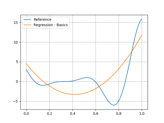
Plotting#
Of course, you can see that the quadratic model is no good at all here:
test_dataset = sample_disciplines(
    [discipline], input_space, "y", algo_name="PYDOE_FULLFACT", n_samples=100
)
input_data = test_dataset.get_view(variable_names=model.input_names).to_numpy()
reference_output_data = test_dataset.get_view(variable_names="y").to_numpy().ravel()
predicted_output_data = model.predict(input_data).ravel()
plt.plot(input_data.ravel(), reference_output_data, label="Reference")
plt.plot(input_data.ravel(), predicted_output_data, label="Regression - Basics")
plt.grid()
plt.legend()
plt.show()
INFO - 16:16:12: *** Start Sampling execution ***
INFO - 16:16:12: Sampling
INFO - 16:16:12:    Disciplines: f
INFO - 16:16:12:    MDO formulation: MDF
INFO - 16:16:12: Running the algorithm PYDOE_FULLFACT:
INFO - 16:16:12:      1%|          | 1/100 [00:00<00:00, 4396.55 it/sec]
INFO - 16:16:12:      2%|▏         | 2/100 [00:00<00:00, 3863.94 it/sec]
INFO - 16:16:12:      3%|▎         | 3/100 [00:00<00:00, 3922.35 it/sec]
INFO - 16:16:12:      4%|▍         | 4/100 [00:00<00:00, 3894.43 it/sec]
INFO - 16:16:12:      5%|▌         | 5/100 [00:00<00:00, 3968.87 it/sec]
INFO - 16:16:12:      6%|▌         | 6/100 [00:00<00:00, 4036.87 it/sec]
INFO - 16:16:12:      7%|▋         | 7/100 [00:00<00:00, 4082.33 it/sec]
INFO - 16:16:12:      8%|▊         | 8/100 [00:00<00:00, 4088.51 it/sec]
INFO - 16:16:12:      9%|▉         | 9/100 [00:00<00:00, 4134.13 it/sec]
INFO - 16:16:12:     10%|█         | 10/100 [00:00<00:00, 4170.53 it/sec]
INFO - 16:16:12:     11%|█         | 11/100 [00:00<00:00, 4203.86 it/sec]
INFO - 16:16:12:     12%|█▏        | 12/100 [00:00<00:00, 4236.67 it/sec]
INFO - 16:16:12:     13%|█▎        | 13/100 [00:00<00:00, 4214.73 it/sec]
INFO - 16:16:12:     14%|█▍        | 14/100 [00:00<00:00, 4242.18 it/sec]
INFO - 16:16:12:     15%|█▌        | 15/100 [00:00<00:00, 4264.24 it/sec]
INFO - 16:16:12:     16%|█▌        | 16/100 [00:00<00:00, 4288.11 it/sec]
INFO - 16:16:12:     17%|█▋        | 17/100 [00:00<00:00, 4288.91 it/sec]
INFO - 16:16:12:     18%|█▊        | 18/100 [00:00<00:00, 4306.76 it/sec]
INFO - 16:16:12:     19%|█▉        | 19/100 [00:00<00:00, 4310.46 it/sec]
INFO - 16:16:12:     20%|██        | 20/100 [00:00<00:00, 4328.93 it/sec]
INFO - 16:16:12:     21%|██        | 21/100 [00:00<00:00, 4345.36 it/sec]
INFO - 16:16:12:     22%|██▏       | 22/100 [00:00<00:00, 4337.44 it/sec]
INFO - 16:16:12:     23%|██▎       | 23/100 [00:00<00:00, 4352.31 it/sec]
INFO - 16:16:12:     24%|██▍       | 24/100 [00:00<00:00, 4369.07 it/sec]
INFO - 16:16:12:     25%|██▌       | 25/100 [00:00<00:00, 4383.13 it/sec]
INFO - 16:16:12:     26%|██▌       | 26/100 [00:00<00:00, 4381.18 it/sec]
INFO - 16:16:12:     27%|██▋       | 27/100 [00:00<00:00, 4391.09 it/sec]
INFO - 16:16:12:     28%|██▊       | 28/100 [00:00<00:00, 4400.17 it/sec]
INFO - 16:16:12:     29%|██▉       | 29/100 [00:00<00:00, 4410.57 it/sec]
INFO - 16:16:12:     30%|███       | 30/100 [00:00<00:00, 4421.26 it/sec]
INFO - 16:16:12:     31%|███       | 31/100 [00:00<00:00, 4412.21 it/sec]
INFO - 16:16:12:     32%|███▏      | 32/100 [00:00<00:00, 4419.85 it/sec]
INFO - 16:16:12:     33%|███▎      | 33/100 [00:00<00:00, 4427.91 it/sec]
INFO - 16:16:12:     34%|███▍      | 34/100 [00:00<00:00, 4438.56 it/sec]
INFO - 16:16:12:     35%|███▌      | 35/100 [00:00<00:00, 4436.94 it/sec]
INFO - 16:16:12:     36%|███▌      | 36/100 [00:00<00:00, 4437.50 it/sec]
INFO - 16:16:12:     37%|███▋      | 37/100 [00:00<00:00, 4440.45 it/sec]
INFO - 16:16:12:     38%|███▊      | 38/100 [00:00<00:00, 4447.58 it/sec]
INFO - 16:16:12:     39%|███▉      | 39/100 [00:00<00:00, 4453.76 it/sec]
INFO - 16:16:12:     40%|████      | 40/100 [00:00<00:00, 4450.19 it/sec]
INFO - 16:16:12:     41%|████      | 41/100 [00:00<00:00, 4455.55 it/sec]
INFO - 16:16:12:     42%|████▏     | 42/100 [00:00<00:00, 4461.46 it/sec]
INFO - 16:16:12:     43%|████▎     | 43/100 [00:00<00:00, 4466.67 it/sec]
INFO - 16:16:12:     44%|████▍     | 44/100 [00:00<00:00, 4472.30 it/sec]
INFO - 16:16:12:     45%|████▌     | 45/100 [00:00<00:00, 4466.46 it/sec]
INFO - 16:16:12:     46%|████▌     | 46/100 [00:00<00:00, 4470.40 it/sec]
INFO - 16:16:12:     47%|████▋     | 47/100 [00:00<00:00, 4474.48 it/sec]
INFO - 16:16:12:     48%|████▊     | 48/100 [00:00<00:00, 4480.10 it/sec]
INFO - 16:16:12:     49%|████▉     | 49/100 [00:00<00:00, 4476.02 it/sec]
INFO - 16:16:12:     50%|█████     | 50/100 [00:00<00:00, 4479.08 it/sec]
INFO - 16:16:12:     51%|█████     | 51/100 [00:00<00:00, 4483.82 it/sec]
INFO - 16:16:12:     52%|█████▏    | 52/100 [00:00<00:00, 4488.56 it/sec]
INFO - 16:16:12:     53%|█████▎    | 53/100 [00:00<00:00, 4493.23 it/sec]
INFO - 16:16:12:     54%|█████▍    | 54/100 [00:00<00:00, 4487.75 it/sec]
INFO - 16:16:12:     55%|█████▌    | 55/100 [00:00<00:00, 4489.99 it/sec]
INFO - 16:16:12:     56%|█████▌    | 56/100 [00:00<00:00, 4489.66 it/sec]
INFO - 16:16:12:     57%|█████▋    | 57/100 [00:00<00:00, 4494.49 it/sec]
INFO - 16:16:12:     58%|█████▊    | 58/100 [00:00<00:00, 4491.85 it/sec]
INFO - 16:16:12:     59%|█████▉    | 59/100 [00:00<00:00, 4494.69 it/sec]
INFO - 16:16:12:     60%|██████    | 60/100 [00:00<00:00, 4499.20 it/sec]
INFO - 16:16:12:     61%|██████    | 61/100 [00:00<00:00, 4471.93 it/sec]
INFO - 16:16:12:     62%|██████▏   | 62/100 [00:00<00:00, 4465.86 it/sec]
INFO - 16:16:12:     63%|██████▎   | 63/100 [00:00<00:00, 4464.14 it/sec]
INFO - 16:16:12:     64%|██████▍   | 64/100 [00:00<00:00, 4465.74 it/sec]
INFO - 16:16:12:     65%|██████▌   | 65/100 [00:00<00:00, 4468.39 it/sec]
INFO - 16:16:12:     66%|██████▌   | 66/100 [00:00<00:00, 4471.68 it/sec]
INFO - 16:16:12:     67%|██████▋   | 67/100 [00:00<00:00, 4468.84 it/sec]
INFO - 16:16:12:     68%|██████▊   | 68/100 [00:00<00:00, 4472.73 it/sec]
INFO - 16:16:12:     69%|██████▉   | 69/100 [00:00<00:00, 4476.31 it/sec]
INFO - 16:16:12:     70%|███████   | 70/100 [00:00<00:00, 4480.00 it/sec]
INFO - 16:16:12:     71%|███████   | 71/100 [00:00<00:00, 4483.12 it/sec]
INFO - 16:16:12:     72%|███████▏  | 72/100 [00:00<00:00, 4477.84 it/sec]
INFO - 16:16:12:     73%|███████▎  | 73/100 [00:00<00:00, 4480.31 it/sec]
INFO - 16:16:12:     74%|███████▍  | 74/100 [00:00<00:00, 4480.51 it/sec]
INFO - 16:16:12:     75%|███████▌  | 75/100 [00:00<00:00, 4483.52 it/sec]
INFO - 16:16:12:     76%|███████▌  | 76/100 [00:00<00:00, 4481.28 it/sec]
INFO - 16:16:12:     77%|███████▋  | 77/100 [00:00<00:00, 4481.84 it/sec]
INFO - 16:16:12:     78%|███████▊  | 78/100 [00:00<00:00, 4484.53 it/sec]
INFO - 16:16:12:     79%|███████▉  | 79/100 [00:00<00:00, 4486.62 it/sec]
INFO - 16:16:12:     80%|████████  | 80/100 [00:00<00:00, 4489.43 it/sec]
INFO - 16:16:12:     81%|████████  | 81/100 [00:00<00:00, 4484.70 it/sec]
INFO - 16:16:12:     82%|████████▏ | 82/100 [00:00<00:00, 4486.94 it/sec]
INFO - 16:16:12:     83%|████████▎ | 83/100 [00:00<00:00, 4488.55 it/sec]
INFO - 16:16:12:     84%|████████▍ | 84/100 [00:00<00:00, 4491.26 it/sec]
INFO - 16:16:12:     85%|████████▌ | 85/100 [00:00<00:00, 4489.84 it/sec]
INFO - 16:16:12:     86%|████████▌ | 86/100 [00:00<00:00, 4490.47 it/sec]
INFO - 16:16:12:     87%|████████▋ | 87/100 [00:00<00:00, 4492.13 it/sec]
INFO - 16:16:12:     88%|████████▊ | 88/100 [00:00<00:00, 4493.92 it/sec]
INFO - 16:16:12:     89%|████████▉ | 89/100 [00:00<00:00, 4496.15 it/sec]
INFO - 16:16:12:     90%|█████████ | 90/100 [00:00<00:00, 4493.15 it/sec]
INFO - 16:16:12:     91%|█████████ | 91/100 [00:00<00:00, 4495.50 it/sec]
INFO - 16:16:12:     92%|█████████▏| 92/100 [00:00<00:00, 4494.98 it/sec]
INFO - 16:16:12:     93%|█████████▎| 93/100 [00:00<00:00, 4496.95 it/sec]
INFO - 16:16:12:     94%|█████████▍| 94/100 [00:00<00:00, 4494.89 it/sec]
INFO - 16:16:12:     95%|█████████▌| 95/100 [00:00<00:00, 4495.86 it/sec]
INFO - 16:16:12:     96%|█████████▌| 96/100 [00:00<00:00, 4498.47 it/sec]
INFO - 16:16:12:     97%|█████████▋| 97/100 [00:00<00:00, 4499.88 it/sec]
INFO - 16:16:12:     98%|█████████▊| 98/100 [00:00<00:00, 4502.10 it/sec]
INFO - 16:16:12:     99%|█████████▉| 99/100 [00:00<00:00, 4499.50 it/sec]
INFO - 16:16:12:    100%|██████████| 100/100 [00:00<00:00, 4448.44 it/sec]
INFO - 16:16:12: *** End Sampling execution ***
Settings#
The PolynomialRegressor has many options
defined in the PolynomialRegressor_Settings Pydantic model.
Most of them are presented
in the example about the linear regression model.
The only one we will look at here is the degree of the polynomial regression model.
This information can be set with the degree keyword.
For example,
we can use a cubic regression model instead of a quadratic one:
model = create_regression_model("PolynomialRegressor", training_dataset, degree=3)
model.learn()
and see that this model seems to be better:
predicted_output_data_ = model.predict(input_data).ravel()
plt.plot(input_data.ravel(), reference_output_data, label="Reference")
plt.plot(input_data.ravel(), predicted_output_data, label="Regression - Basics")
plt.plot(input_data.ravel(), predicted_output_data_, label="Regression - Degree(3)")
plt.grid()
plt.legend()
plt.show()

Total running time of the script: (0 minutes 0.148 seconds)