Note
Go to the end to download the full example code.
Morris analysis#
from __future__ import annotations

import pprint

from gemseo.problems.uncertainty.ishigami.ishigami_discipline import IshigamiDiscipline
from gemseo.problems.uncertainty.ishigami.ishigami_space import IshigamiSpace
from gemseo.uncertainty.sensitivity.morris_analysis import MorrisAnalysis
In this example, we consider the Ishigami function [IH90]
implemented as an Discipline by the IshigamiDiscipline.
It is commonly used
with the independent random variables \(X_1\), \(X_2\) and \(X_3\)
uniformly distributed between \(-\pi\) and \(\pi\)
and defined in the IshigamiSpace.
discipline = IshigamiDiscipline()
uncertain_space = IshigamiSpace()
Then,
we run sensitivity analysis of type MorrisAnalysis:
sensitivity_analysis = MorrisAnalysis()
sensitivity_analysis.compute_samples([discipline], uncertain_space, n_samples=0)
sensitivity_analysis.compute_indices()
INFO - 16:21:58: *** Start MorrisAnalysisSamplingPhase execution ***
INFO - 16:21:58: MorrisAnalysisSamplingPhase
INFO - 16:21:58: Disciplines: IshigamiDiscipline
INFO - 16:21:58: MDO formulation: MDF
INFO - 16:21:58: Running the algorithm MorrisDOE:
INFO - 16:21:58: 5%|▌ | 1/20 [00:00<00:00, 483.77 it/sec]
INFO - 16:21:58: 10%|█ | 2/20 [00:00<00:00, 817.20 it/sec]
INFO - 16:21:58: 15%|█▌ | 3/20 [00:00<00:00, 1090.56 it/sec]
INFO - 16:21:58: 20%|██ | 4/20 [00:00<00:00, 1311.64 it/sec]
INFO - 16:21:58: 25%|██▌ | 5/20 [00:00<00:00, 1498.29 it/sec]
INFO - 16:21:58: 30%|███ | 6/20 [00:00<00:00, 1672.15 it/sec]
INFO - 16:21:58: 35%|███▌ | 7/20 [00:00<00:00, 1816.95 it/sec]
INFO - 16:21:58: 40%|████ | 8/20 [00:00<00:00, 1929.08 it/sec]
INFO - 16:21:58: 45%|████▌ | 9/20 [00:00<00:00, 2045.00 it/sec]
INFO - 16:21:58: 50%|█████ | 10/20 [00:00<00:00, 2154.57 it/sec]
INFO - 16:21:58: 55%|█████▌ | 11/20 [00:00<00:00, 2196.28 it/sec]
INFO - 16:21:58: 60%|██████ | 12/20 [00:00<00:00, 2259.76 it/sec]
INFO - 16:21:58: 65%|██████▌ | 13/20 [00:00<00:00, 2338.46 it/sec]
INFO - 16:21:58: 70%|███████ | 14/20 [00:00<00:00, 2415.28 it/sec]
INFO - 16:21:58: 75%|███████▌ | 15/20 [00:00<00:00, 2479.39 it/sec]
INFO - 16:21:58: 80%|████████ | 16/20 [00:00<00:00, 2524.88 it/sec]
INFO - 16:21:58: 85%|████████▌ | 17/20 [00:00<00:00, 2585.60 it/sec]
INFO - 16:21:58: 90%|█████████ | 18/20 [00:00<00:00, 2641.90 it/sec]
INFO - 16:21:58: 95%|█████████▌| 19/20 [00:00<00:00, 2690.29 it/sec]
INFO - 16:21:58: 100%|██████████| 20/20 [00:00<00:00, 2684.87 it/sec]
INFO - 16:21:58: *** End MorrisAnalysisSamplingPhase execution ***
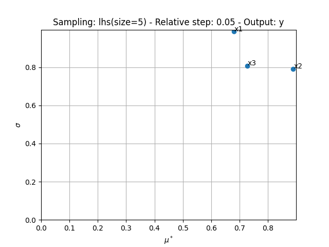
MorrisAnalysis.SensitivityIndices(mu={'y': [{'x1': array([-0.60047199]), 'x2': array([0.51230435]), 'x3': array([-0.89800793])}]}, mu_star={'y': [{'x1': array([0.69887482]), 'x2': array([0.65136343]), 'x3': array([0.89805157])}]}, sigma={'y': [{'x1': array([0.96395158]), 'x2': array([0.6549141]), 'x3': array([0.79878356])}]}, relative_sigma={'y': [{'x1': array([1.37929075]), 'x2': array([1.00545113]), 'x3': array([0.88946291])}]}, min={'y': [{'x1': array([0.0338188]), 'x2': array([0.11821721]), 'x3': array([8.72820113e-05])}]}, max={'y': [{'x1': array([2.2360336]), 'x2': array([1.25769934]), 'x3': array([2.12052546])}]})
The resulting indices are the empirical means and the standard deviations of the absolute output variations due to input changes.
sensitivity_analysis.indices
MorrisAnalysis.SensitivityIndices(mu={'y': [{'x1': array([-0.60047199]), 'x2': array([0.51230435]), 'x3': array([-0.89800793])}]}, mu_star={'y': [{'x1': array([0.69887482]), 'x2': array([0.65136343]), 'x3': array([0.89805157])}]}, sigma={'y': [{'x1': array([0.96395158]), 'x2': array([0.6549141]), 'x3': array([0.79878356])}]}, relative_sigma={'y': [{'x1': array([1.37929075]), 'x2': array([1.00545113]), 'x3': array([0.88946291])}]}, min={'y': [{'x1': array([0.0338188]), 'x2': array([0.11821721]), 'x3': array([8.72820113e-05])}]}, max={'y': [{'x1': array([2.2360336]), 'x2': array([1.25769934]), 'x3': array([2.12052546])}]})
The main indices corresponds to these empirical means
(this main method can be changed with MorrisAnalysis.main_method):
pprint.pprint(sensitivity_analysis.main_indices)
{'y': [{'x1': array([0.69887482]),
        'x2': array([0.65136343]),
        'x3': array([0.89805157])}]}
and can be interpreted with respect to the empirical bounds of the outputs:
pprint.pprint(sensitivity_analysis.outputs_bounds)
{'y': (array([-1.42959705]), array([14.89344259]))}
We can also get the input parameters sorted by decreasing order of influence:
sensitivity_analysis.sort_input_variables("y")
['x3', 'x1', 'x2']
We can use the method MorrisAnalysis.plot()
to visualize the different series of indices:
sensitivity_analysis.plot("y", save=False, show=True, lower_mu=0, lower_sigma=0)
<Figure size 640x480 with 1 Axes>
Lastly,
the sensitivity indices can be exported to a Dataset:
sensitivity_analysis.to_dataset()
Total running time of the script: (0 minutes 0.088 seconds)