Quadratic approximations

In this example, we illustrate the use of the QuadApprox plot on the Sobieski’s SSBJ problem.

from gemseo.api import configure_logger
from gemseo.api import create_discipline
from gemseo.api import create_scenario
from gemseo.problems.sobieski.core.problem import SobieskiProblem
from matplotlib import pyplot as plt

Import

The first step is to import some functions from the API and a method to get the design space.

configure_logger()

Out:

<RootLogger root (INFO)>

Description

The QuadApprox post-processing performs a quadratic approximation of a given function from an optimization history and plot the results as cuts of the approximation.

Create disciplines

Then, we instantiate the disciplines of the Sobieski’s SSBJ problem: Propulsion, Aerodynamics, Structure and Mission

disciplines = create_discipline(
    [
        "SobieskiPropulsion",
        "SobieskiAerodynamics",
        "SobieskiStructure",
        "SobieskiMission",
    ]
)

Create design space

We also read the design space from the SobieskiProblem.

design_space = SobieskiProblem().design_space

Create and execute scenario

The next step is to build an MDO scenario in order to maximize the range, encoded ‘y_4’, with respect to the design parameters, while satisfying the inequality constraints ‘g_1’, ‘g_2’ and ‘g_3’. We can use the MDF formulation, the SLSQP optimization algorithm and a maximum number of iterations equal to 100.

scenario = create_scenario(
    disciplines,
    formulation="MDF",
    objective_name="y_4",
    maximize_objective=True,
    design_space=design_space,
)
scenario.set_differentiation_method("user")
for constraint in ["g_1", "g_2", "g_3"]:
    scenario.add_constraint(constraint, "ineq")
scenario.execute({"algo": "SLSQP", "max_iter": 10})

Out:

    INFO - 10:03:01:
    INFO - 10:03:01: *** Start MDOScenario execution ***
    INFO - 10:03:01: MDOScenario
    INFO - 10:03:01:    Disciplines: SobieskiPropulsion SobieskiAerodynamics SobieskiStructure SobieskiMission
    INFO - 10:03:01:    MDO formulation: MDF
    INFO - 10:03:01: Optimization problem:
    INFO - 10:03:01:    minimize -y_4(x_shared, x_1, x_2, x_3)
    INFO - 10:03:01:    with respect to x_1, x_2, x_3, x_shared
    INFO - 10:03:01:    subject to constraints:
    INFO - 10:03:01:       g_1(x_shared, x_1, x_2, x_3) <= 0.0
    INFO - 10:03:01:       g_2(x_shared, x_1, x_2, x_3) <= 0.0
    INFO - 10:03:01:       g_3(x_shared, x_1, x_2, x_3) <= 0.0
    INFO - 10:03:01:    over the design space:
    INFO - 10:03:01:    +----------+-------------+-------+-------------+-------+
    INFO - 10:03:01:    | name     | lower_bound | value | upper_bound | type  |
    INFO - 10:03:01:    +----------+-------------+-------+-------------+-------+
    INFO - 10:03:01:    | x_shared |     0.01    |  0.05 |     0.09    | float |
    INFO - 10:03:01:    | x_shared |    30000    | 45000 |    60000    | float |
    INFO - 10:03:01:    | x_shared |     1.4     |  1.6  |     1.8     | float |
    INFO - 10:03:01:    | x_shared |     2.5     |  5.5  |     8.5     | float |
    INFO - 10:03:01:    | x_shared |      40     |   55  |      70     | float |
    INFO - 10:03:01:    | x_shared |     500     |  1000 |     1500    | float |
    INFO - 10:03:01:    | x_1      |     0.1     |  0.25 |     0.4     | float |
    INFO - 10:03:01:    | x_1      |     0.75    |   1   |     1.25    | float |
    INFO - 10:03:01:    | x_2      |     0.75    |   1   |     1.25    | float |
    INFO - 10:03:01:    | x_3      |     0.1     |  0.5  |      1      | float |
    INFO - 10:03:01:    +----------+-------------+-------+-------------+-------+
    INFO - 10:03:01: Solving optimization problem with algorithm SLSQP:
    INFO - 10:03:01: ...   0%|          | 0/10 [00:00<?, ?it]
    INFO - 10:03:01: ...  20%|██        | 2/10 [00:00<00:00, 41.39 it/sec, obj=-2.12e+3]
    INFO - 10:03:01: ...  30%|███       | 3/10 [00:00<00:00, 24.85 it/sec, obj=-3.15e+3]
    INFO - 10:03:01: ...  40%|████      | 4/10 [00:00<00:00, 17.71 it/sec, obj=-3.96e+3]
    INFO - 10:03:01: ...  50%|█████     | 5/10 [00:00<00:00, 13.77 it/sec, obj=-3.98e+3]
    INFO - 10:03:01: ...  50%|█████     | 5/10 [00:00<00:00, 12.39 it/sec, obj=-3.98e+3]
    INFO - 10:03:01: Optimization result:
    INFO - 10:03:01:    Optimizer info:
    INFO - 10:03:01:       Status: 8
    INFO - 10:03:01:       Message: Positive directional derivative for linesearch
    INFO - 10:03:01:       Number of calls to the objective function by the optimizer: 6
    INFO - 10:03:01:    Solution:
    INFO - 10:03:01:       The solution is feasible.
    INFO - 10:03:01:       Objective: -3960.1367790933214
    INFO - 10:03:01:       Standardized constraints:
    INFO - 10:03:01:          g_1 = [-0.01805983 -0.03334555 -0.04424879 -0.05183405 -0.05732561 -0.13720865
    INFO - 10:03:01:  -0.10279135]
    INFO - 10:03:01:          g_2 = 2.9360600315442298e-06
    INFO - 10:03:01:          g_3 = [-0.76310174 -0.23689826 -0.00553375 -0.183255  ]
    INFO - 10:03:01:       Design space:
    INFO - 10:03:01:       +----------+-------------+---------------------+-------------+-------+
    INFO - 10:03:01:       | name     | lower_bound |        value        | upper_bound | type  |
    INFO - 10:03:01:       +----------+-------------+---------------------+-------------+-------+
    INFO - 10:03:01:       | x_shared |     0.01    | 0.06000073401500788 |     0.09    | float |
    INFO - 10:03:01:       | x_shared |    30000    |        60000        |    60000    | float |
    INFO - 10:03:01:       | x_shared |     1.4     |         1.4         |     1.8     | float |
    INFO - 10:03:01:       | x_shared |     2.5     |         2.5         |     8.5     | float |
    INFO - 10:03:01:       | x_shared |      40     |          70         |      70     | float |
    INFO - 10:03:01:       | x_shared |     500     |         1500        |     1500    | float |
    INFO - 10:03:01:       | x_1      |     0.1     |         0.4         |     0.4     | float |
    INFO - 10:03:01:       | x_1      |     0.75    |         0.75        |     1.25    | float |
    INFO - 10:03:01:       | x_2      |     0.75    |         0.75        |     1.25    | float |
    INFO - 10:03:01:       | x_3      |     0.1     |  0.1553801266337427 |      1      | float |
    INFO - 10:03:01:       +----------+-------------+---------------------+-------------+-------+
    INFO - 10:03:01: *** End MDOScenario execution (time: 0:00:00.820089) ***

{'max_iter': 10, 'algo': 'SLSQP'}

Post-process scenario

Lastly, we post-process the scenario by means of the QuadApprox plot which performs a quadratic approximation of a given function from an optimization history and plot the results as cuts of the approximation.

Tip

Each post-processing method requires different inputs and offers a variety of customization options. Use the API function get_post_processing_options_schema() to print a table with the options for any post-processing algorithm. Or refer to our dedicated page: Post-processing algorithms.

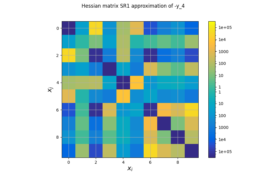
The first plot shows an approximation of the Hessian matrix \(\frac{\partial^2 f}{\partial x_i \partial x_j}\) based on the Symmetric Rank 1 method (SR1) [NW06]. The color map uses a symmetric logarithmic (symlog) scale. This plots the cross influence of the design variables on the objective function or constraints. For instance, on the last figure, the maximal second-order sensitivity is \(\frac{\partial^2 -y_4}{\partial^2 x_0} = 2.10^5\), which means that the \(x_0\) is the most influential variable. Then, the cross derivative \(\frac{\partial^2 -y_4}{\partial x_0 \partial x_2} = 5.10^4\) is positive and relatively high compared to the previous one but the combined effects of \(x_0\) and \(x_2\) are non-negligible in comparison.

scenario.post_process("QuadApprox", function="-y_4", save=False, show=False)
# Workaround for HTML rendering, instead of ``show=True``
plt.show()

• 
• 

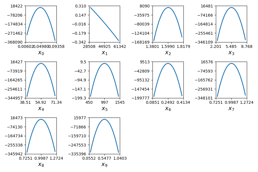
The second plot represents the quadratic approximation of the objective around the optimal solution : \(a_{i}(t)=0.5 (t-x^*_i)^2 \frac{\partial^2 f}{\partial x_i^2} + (t-x^*_i) \frac{\partial f}{\partial x_i} + f(x^*)\), where \(x^*\) is the optimal solution. This approximation highlights the sensitivity of the objective function with respect to the design variables: we notice that the design variables \(x\_1, x\_5, x\_6\) have little influence , whereas \(x\_0, x\_2, x\_9\) have a huge influence on the objective. This trend is also noted in the diagonal terms of the Hessian matrix \(\frac{\partial^2 f}{\partial x_i^2}\).