Note
Go to the end to download the full example code.
MDF-based DOE on the Sobieski SSBJ test case#
from __future__ import annotations

from os import name as os_name

from gemseo import create_discipline
from gemseo import create_scenario
from gemseo import generate_n2_plot
from gemseo.problems.mdo.sobieski.core.design_space import SobieskiDesignSpace
from gemseo.settings.doe import PYDOE_LHS_Settings
Instantiate the disciplines#
First, we instantiate the four disciplines of the use case:
SobieskiPropulsion,
SobieskiAerodynamics,
SobieskiMission
and SobieskiStructure.
disciplines = create_discipline([
    "SobieskiPropulsion",
    "SobieskiAerodynamics",
    "SobieskiMission",
    "SobieskiStructure",
])
We can quickly access the most relevant information of any discipline (name, inputs,
and outputs) with Python's print() function. Moreover, we can get the default
input values of a discipline with the attribute Discipline.default_input_data
for discipline in disciplines:
    print(discipline)
    print(f"Default inputs: {discipline.default_input_data}")
SobieskiPropulsion
Default inputs: {'y_23': array([12562.01206488]), 'x_3': array([0.5]), 'x_shared': array([5.0e-02, 4.5e+04, 1.6e+00, 5.5e+00, 5.5e+01, 1.0e+03]), 'c_3': array([4360.])}
SobieskiAerodynamics
Default inputs: {'x_2': array([1.]), 'y_32': array([0.50279625]), 'x_shared': array([5.0e-02, 4.5e+04, 1.6e+00, 5.5e+00, 5.5e+01, 1.0e+03]), 'y_12': array([5.06069742e+04, 9.50000000e-01]), 'c_4': array([0.01375])}
SobieskiMission
Default inputs: {'y_14': array([50606.9741711 ,  7306.20262124]), 'x_shared': array([5.0e-02, 4.5e+04, 1.6e+00, 5.5e+00, 5.5e+01, 1.0e+03]), 'y_24': array([4.15006276]), 'y_34': array([1.10754577])}
SobieskiStructure
Default inputs: {'y_21': array([50606.9741711]), 'y_31': array([6354.32430691]), 'x_1': array([0.25, 1.  ]), 'x_shared': array([5.0e-02, 4.5e+04, 1.6e+00, 5.5e+00, 5.5e+01, 1.0e+03]), 'c_0': array([2000.]), 'c_1': array([25000.]), 'c_2': array([6.])}
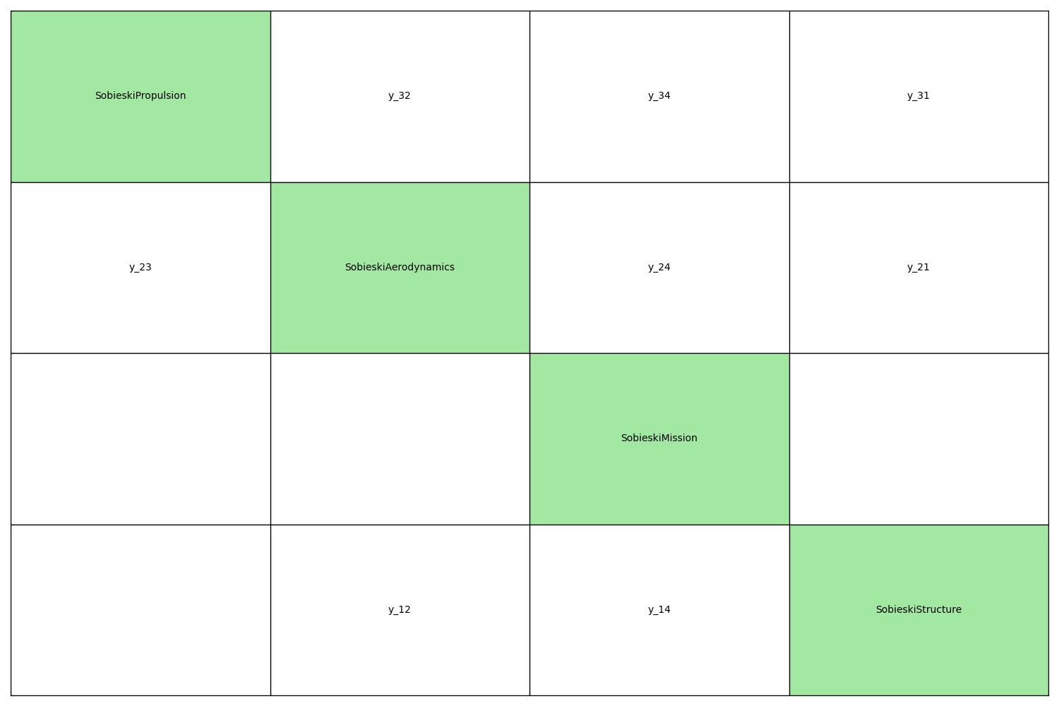
You may also be interested in plotting the couplings of your disciplines.
A quick way of getting this information is the high-level function
generate_n2_plot(). A much more detailed explanation of coupling
visualization is available here.
generate_n2_plot(disciplines, save=False, show=True)
Build, execute and post-process the scenario#
Then, we build the scenario which links the disciplines
with the formulation and the optimization algorithm. Here, we use the
BiLevel formulation. We tell the scenario to minimize -y_4
instead of minimizing y_4 (range), which is the default option.
We need to define the design space.
design_space = SobieskiDesignSpace()
design_space
Instantiate the scenario#
scenario = create_scenario(
    disciplines,
    "y_4",
    design_space,
    maximize_objective=True,
    scenario_type="DOE",
    formulation_name="MDF",
)
Set the design constraints#
for constraint in ["g_1", "g_2", "g_3"]:
    scenario.add_constraint(constraint, constraint_type="ineq")
Visualize the XDSM#
Generate the XDSM on the fly:
log_workflow_status=Truewill log the status of the workflow in the console,save_html(defaultTrue) will generate a self-contained HTML file, that can be automatically opened usingshow_html=True.
scenario.xdsmize(save_html=False)
Execute the scenario#
Use provided analytic derivatives
scenario.set_differentiation_method()
Multiprocessing#
It is possible to run a DOE in parallel using multiprocessing, in order to do this, we specify the number of processes to be used for the computation of the samples.
Warning
The multiprocessing option has some limitations on Windows.
Due to problems with sphinx, we disable it in this example.
The features MemoryFullCache and HDF5Cache are not
available for multiprocessing on Windows.
As an alternative, we recommend the method
DOEScenario.set_optimization_history_backup().
We define the algorithm settings. Here the criterion "center" of pyDOE centers the points within the sampling intervals. Note that it is also possible to pass the settings one by one, see Algorithm Settings.
lhs_settings = PYDOE_LHS_Settings(
    n_samples=30,
    criterion="center",
    # Evaluate gradient of the MDA
    # with coupled adjoint
    eval_jac=True,
    # Run in parallel on 1 or 4 processors
    n_processes=1 if os_name == "nt" else 4,
)

scenario.execute(lhs_settings)
INFO - 16:13:45: *** Start DOEScenario execution ***
INFO - 16:13:45: DOEScenario
INFO - 16:13:45:    Disciplines: SobieskiAerodynamics SobieskiMission SobieskiPropulsion SobieskiStructure
INFO - 16:13:45:    MDO formulation: MDF
INFO - 16:13:45: Optimization problem:
INFO - 16:13:45:    minimize -y_4(x_shared, x_1, x_2, x_3)
INFO - 16:13:45:    with respect to x_1, x_2, x_3, x_shared
INFO - 16:13:45:    under the inequality constraints
INFO - 16:13:45:       g_1(x_shared, x_1, x_2, x_3) <= 0
INFO - 16:13:45:       g_2(x_shared, x_1, x_2, x_3) <= 0
INFO - 16:13:45:       g_3(x_shared, x_1, x_2, x_3) <= 0
INFO - 16:13:45:    over the design space:
INFO - 16:13:45:       +-------------+-------------+-------+-------------+-------+
INFO - 16:13:45:       | Name        | Lower bound | Value | Upper bound | Type  |
INFO - 16:13:45:       +-------------+-------------+-------+-------------+-------+
INFO - 16:13:45:       | x_shared[0] |     0.01    |  0.05 |     0.09    | float |
INFO - 16:13:45:       | x_shared[1] |    30000    | 45000 |    60000    | float |
INFO - 16:13:45:       | x_shared[2] |     1.4     |  1.6  |     1.8     | float |
INFO - 16:13:45:       | x_shared[3] |     2.5     |  5.5  |     8.5     | float |
INFO - 16:13:45:       | x_shared[4] |      40     |   55  |      70     | float |
INFO - 16:13:45:       | x_shared[5] |     500     |  1000 |     1500    | float |
INFO - 16:13:45:       | x_1[0]      |     0.1     |  0.25 |     0.4     | float |
INFO - 16:13:45:       | x_1[1]      |     0.75    |   1   |     1.25    | float |
INFO - 16:13:45:       | x_2         |     0.75    |   1   |     1.25    | float |
INFO - 16:13:45:       | x_3         |     0.1     |  0.5  |      1      | float |
INFO - 16:13:45:       +-------------+-------------+-------+-------------+-------+
INFO - 16:13:45: Solving optimization problem with algorithm PYDOE_LHS:
INFO - 16:13:45: Running DOE in parallel on n_processes = 4
INFO - 16:13:45:      3%|▎         | 1/30 [00:00<00:03,  7.53 it/sec, feas=True, obj=-285]
INFO - 16:13:45:      7%|▋         | 2/30 [00:00<00:02, 10.77 it/sec, feas=False, obj=-429]
INFO - 16:13:45:     10%|█         | 3/30 [00:00<00:01, 16.07 it/sec, feas=False, obj=-567]
INFO - 16:13:45:     13%|█▎        | 4/30 [00:00<00:01, 21.10 it/sec, feas=False, obj=-222]
INFO - 16:13:45:     17%|█▋        | 5/30 [00:00<00:00, 25.21 it/sec, feas=False, obj=-344]
INFO - 16:13:45:     20%|██        | 6/30 [00:00<00:00, 25.05 it/sec, feas=False, obj=-235]
INFO - 16:13:45:     23%|██▎       | 7/30 [00:00<00:00, 29.16 it/sec, feas=False, obj=-519]
INFO - 16:13:45:     27%|██▋       | 8/30 [00:00<00:00, 31.67 it/sec, feas=False, obj=-481]
INFO - 16:13:45:     30%|███       | 9/30 [00:00<00:00, 34.33 it/sec, feas=False, obj=-538]
INFO - 16:13:45:     33%|███▎      | 10/30 [00:00<00:00, 35.39 it/sec, feas=False, obj=-306]
INFO - 16:13:45:     37%|███▋      | 11/30 [00:00<00:00, 37.27 it/sec, feas=False, obj=-419]
INFO - 16:13:45:     40%|████      | 12/30 [00:00<00:00, 40.51 it/sec, feas=False, obj=-556]
INFO - 16:13:45:     43%|████▎     | 13/30 [00:00<00:00, 39.41 it/sec, feas=False, obj=-433]
INFO - 16:13:45:     47%|████▋     | 14/30 [00:00<00:00, 42.36 it/sec, feas=False, obj=-495]
INFO - 16:13:45:     50%|█████     | 15/30 [00:00<00:00, 44.06 it/sec, feas=False, obj=-621]
INFO - 16:13:45:     53%|█████▎    | 16/30 [00:00<00:00, 44.57 it/sec, feas=False, obj=-574]
INFO - 16:13:45:     57%|█████▋    | 17/30 [00:00<00:00, 45.23 it/sec, feas=False, obj=-287]
INFO - 16:13:45:     60%|██████    | 18/30 [00:00<00:00, 46.27 it/sec, feas=False, obj=-481]
INFO - 16:13:46:     63%|██████▎   | 19/30 [00:00<00:00, 48.22 it/sec, feas=False, obj=-1.07e+3]
INFO - 16:13:46:     67%|██████▋   | 20/30 [00:00<00:00, 48.34 it/sec, feas=False, obj=-247]
INFO - 16:13:46:     70%|███████   | 21/30 [00:00<00:00, 50.63 it/sec, feas=False, obj=-602]
INFO - 16:13:46:     73%|███████▎  | 22/30 [00:00<00:00, 49.59 it/sec, feas=False, obj=-414]
INFO - 16:13:46:     77%|███████▋  | 23/30 [00:00<00:00, 50.38 it/sec, feas=False, obj=-273]
INFO - 16:13:46:     80%|████████  | 24/30 [00:00<00:00, 50.98 it/sec, feas=False, obj=-1.18e+3]
INFO - 16:13:46:     83%|████████▎ | 25/30 [00:00<00:00, 51.69 it/sec, feas=False, obj=-383]
INFO - 16:13:46:     87%|████████▋ | 26/30 [00:00<00:00, 53.67 it/sec, feas=False, obj=-624]
INFO - 16:13:46:     90%|█████████ | 27/30 [00:00<00:00, 53.85 it/sec, feas=False, obj=-606]
INFO - 16:13:46:     93%|█████████▎| 28/30 [00:00<00:00, 53.28 it/sec, feas=True, obj=-485]
INFO - 16:13:46:     97%|█████████▋| 29/30 [00:00<00:00, 54.76 it/sec, feas=False, obj=-351]
INFO - 16:13:46:    100%|██████████| 30/30 [00:00<00:00, 56.31 it/sec, feas=False, obj=-405]
INFO - 16:13:46: Optimization result:
INFO - 16:13:46:    Optimizer info:
INFO - 16:13:46:       Status: None
INFO - 16:13:46:       Message: None
INFO - 16:13:46:    Solution:
INFO - 16:13:46:       The solution is feasible.
INFO - 16:13:46:       Objective: -485.49213288049987
INFO - 16:13:46:       Standardized constraints:
INFO - 16:13:46:          g_1 = [-0.11350951 -0.10812292 -0.1045109  -0.10204971 -0.10028641 -0.01838903
INFO - 16:13:46:  -0.22161097]
INFO - 16:13:46:          g_2 = -0.02400000000000002
INFO - 16:13:46:          g_3 = [-0.33063169 -0.66936831 -0.73821755 -0.07789536]
INFO - 16:13:46:       Design space:
INFO - 16:13:46:          +-------------+-------------+---------------------+-------------+-------+
INFO - 16:13:46:          | Name        | Lower bound |        Value        | Upper bound | Type  |
INFO - 16:13:46:          +-------------+-------------+---------------------+-------------+-------+
INFO - 16:13:46:          | x_shared[0] |     0.01    | 0.05400000000000001 |     0.09    | float |
INFO - 16:13:46:          | x_shared[1] |    30000    |        46500        |    60000    | float |
INFO - 16:13:46:          | x_shared[2] |     1.4     |  1.686666666666667  |     1.8     | float |
INFO - 16:13:46:          | x_shared[3] |     2.5     |         5.2         |     8.5     | float |
INFO - 16:13:46:          | x_shared[4] |      40     |         66.5        |      70     | float |
INFO - 16:13:46:          | x_shared[5] |     500     |  583.3333333333334  |     1500    | float |
INFO - 16:13:46:          | x_1[0]      |     0.1     |        0.185        |     0.4     | float |
INFO - 16:13:46:          | x_1[1]      |     0.75    |  0.9416666666666667 |     1.25    | float |
INFO - 16:13:46:          | x_2         |     0.75    |        0.775        |     1.25    | float |
INFO - 16:13:46:          | x_3         |     0.1     |        0.115        |      1      | float |
INFO - 16:13:46:          +-------------+-------------+---------------------+-------------+-------+
INFO - 16:13:46: *** End DOEScenario execution ***
Warning
On Windows, the progress bar may show duplicated instances during the initialization of each subprocess. In some cases it may also print the conclusion of an iteration ahead of another one that was concluded first. This is a consequence of the pickling process and does not affect the computations of the scenario.
Exporting the problem data.#
After the execution of the scenario, you may want to export your data to use it
elsewhere. The method Scenario.to_dataset() will allow you to export
your results to a Dataset, the basic GEMSEO class to store data.
dataset = scenario.to_dataset("a_name_for_my_dataset")
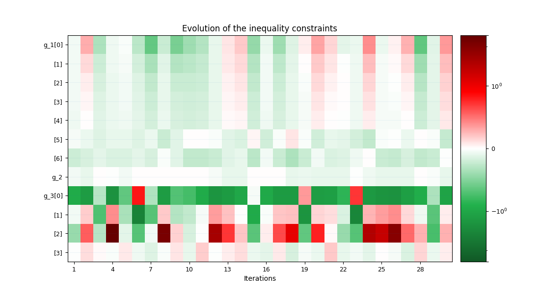
Plot the optimization history view#
scenario.post_process(post_name="OptHistoryView", save=False, show=True)
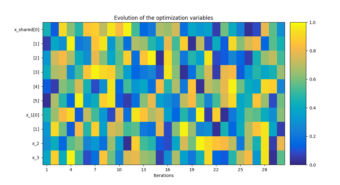
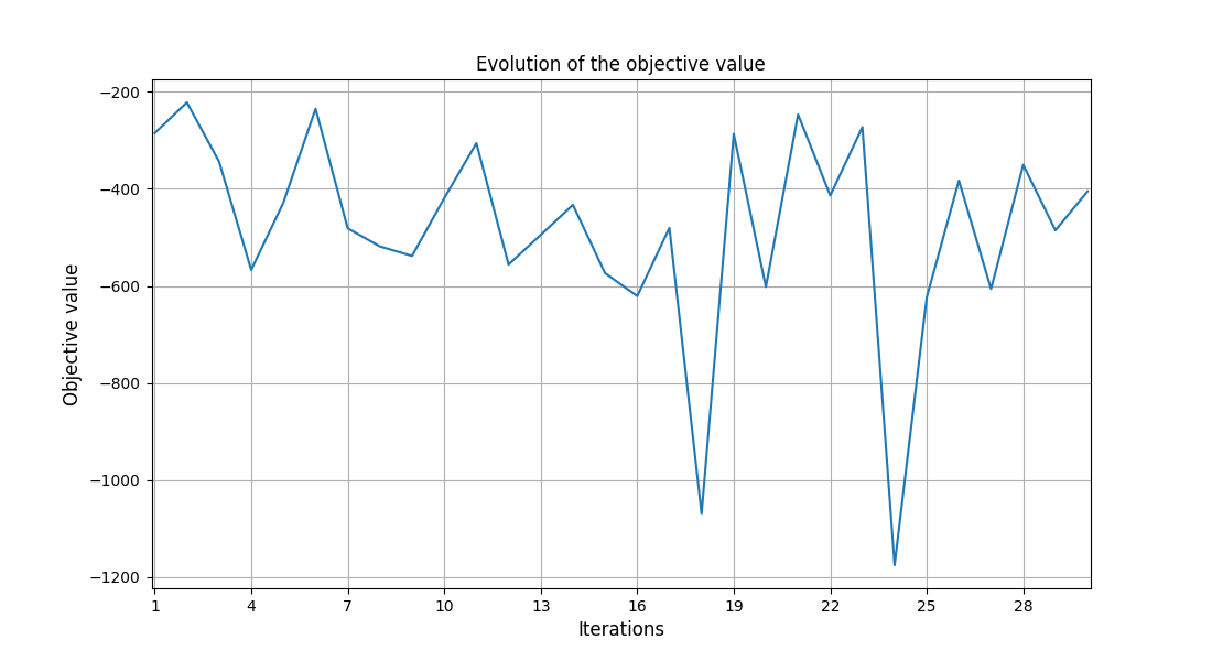
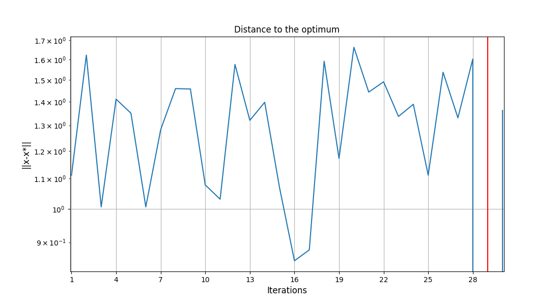
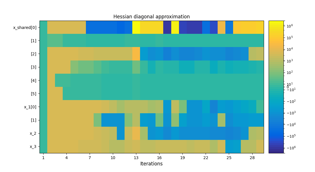
<gemseo.post.opt_history_view.OptHistoryView object at 0x7c4bb2904b00>
Tip
Each post-processing method requires different inputs and offers a variety
of customization options. Use the high-level function
get_post_processing_options_schema() to print a table with
the attributes for any post-processing algo. Or refer to our dedicated page:
Post-processing algorithms.
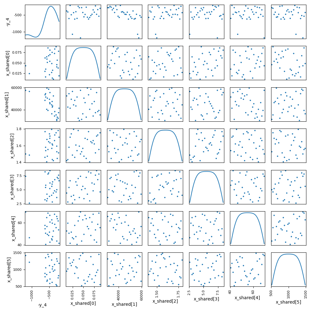
Plot the scatter matrix#
scenario.post_process(
    post_name="ScatterPlotMatrix",
    save=False,
    show=True,
    variable_names=["y_4", "x_shared"],
)
<gemseo.post.scatter_plot_matrix.ScatterPlotMatrix object at 0x7c4bb5ad8dd0>
Plot correlations#
scenario.post_process(post_name="Correlations", save=False, show=True)
    INFO - 16:13:47: Detected 10 correlations > 0.95

<gemseo.post.correlations.Correlations object at 0x7c4bbce24560>
Total running time of the script: (0 minutes 2.761 seconds)