Polynomial chaos expansion (PCE)

A PCERegressor is a PCE model based on OpenTURNS.

from __future__ import annotations

from matplotlib import pyplot as plt
from numpy import array

from gemseo import create_discipline
from gemseo import create_parameter_space
from gemseo import sample_disciplines
from gemseo.mlearning import create_regression_model

Problem

In this example, we represent the function \(f(x)=(6x-2)^2\sin(12x-4)\) [FSK08] by the AnalyticDiscipline

discipline = create_discipline(
    "AnalyticDiscipline",
    name="f",
    expressions={"y": "(6*x-2)**2*sin(12*x-4)"},
)

and seek to approximate it over the input space

input_space = create_parameter_space()
input_space.add_random_variable("x", "OTUniformDistribution")

To do this, we create a training dataset with 6 equispaced points:

training_dataset = sample_disciplines(
    [discipline], input_space, "y", algo_name="PYDOE_FULLFACT", n_samples=10
)

INFO - 16:21:48: *** Start Sampling execution ***
INFO - 16:21:48: Sampling
INFO - 16:21:48:    Disciplines: f
INFO - 16:21:48:    MDO formulation: MDF
INFO - 16:21:48: Running the algorithm PYDOE_FULLFACT:
INFO - 16:21:48:     10%|█         | 1/10 [00:00<00:00, 685.68 it/sec]
INFO - 16:21:48:     20%|██        | 2/10 [00:00<00:00, 1112.84 it/sec]
INFO - 16:21:48:     30%|███       | 3/10 [00:00<00:00, 1451.65 it/sec]
INFO - 16:21:48:     40%|████      | 4/10 [00:00<00:00, 1717.57 it/sec]
INFO - 16:21:48:     50%|█████     | 5/10 [00:00<00:00, 1946.31 it/sec]
INFO - 16:21:48:     60%|██████    | 6/10 [00:00<00:00, 2143.05 it/sec]
INFO - 16:21:48:     70%|███████   | 7/10 [00:00<00:00, 2312.91 it/sec]
INFO - 16:21:48:     80%|████████  | 8/10 [00:00<00:00, 2442.63 it/sec]
INFO - 16:21:48:     90%|█████████ | 9/10 [00:00<00:00, 2566.72 it/sec]
INFO - 16:21:48:    100%|██████████| 10/10 [00:00<00:00, 2618.66 it/sec]
INFO - 16:21:48: *** End Sampling execution ***

Basics

Training

Then, we train an PCE regression model from these samples:

model = create_regression_model("PCERegressor", training_dataset)
model.learn()

WARNING - 16:21:48: Remove input data transformation because PCERegressor does not support transformers.

Prediction

Once it is built, we can predict the output value of \(f\) at a new input point:

input_value = {"x": array([0.65])}
output_value = model.predict(input_value)
output_value

{'y': array([-0.81106394])}

as well as its Jacobian value:

jacobian_value = model.predict_jacobian(input_value)
jacobian_value

{'y': {'x': array([[18.2279622]])}}

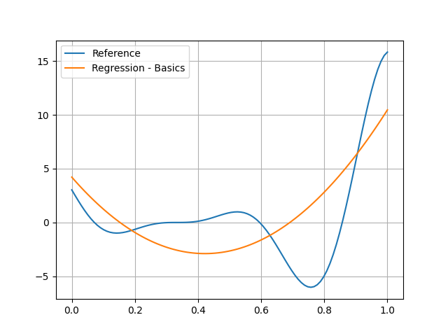
Plotting

Of course, you can see that the quadratic model is no good at all here:

test_dataset = sample_disciplines(
    [discipline], input_space, "y", algo_name="PYDOE_FULLFACT", n_samples=100
)
input_data = test_dataset.get_view(variable_names=model.input_names).to_numpy()
reference_output_data = test_dataset.get_view(variable_names="y").to_numpy().ravel()
predicted_output_data = model.predict(input_data).ravel()
plt.plot(input_data.ravel(), reference_output_data, label="Reference")
plt.plot(input_data.ravel(), predicted_output_data, label="Regression - Basics")
plt.grid()
plt.legend()
plt.show()

INFO - 16:21:48: *** Start Sampling execution ***
INFO - 16:21:48: Sampling
INFO - 16:21:48:    Disciplines: f
INFO - 16:21:48:    MDO formulation: MDF
INFO - 16:21:48: Running the algorithm PYDOE_FULLFACT:
INFO - 16:21:48:      1%|          | 1/100 [00:00<00:00, 3715.06 it/sec]
INFO - 16:21:48:      2%|▏         | 2/100 [00:00<00:00, 3556.00 it/sec]
INFO - 16:21:48:      3%|▎         | 3/100 [00:00<00:00, 3670.63 it/sec]
INFO - 16:21:48:      4%|▍         | 4/100 [00:00<00:00, 3790.60 it/sec]
INFO - 16:21:48:      5%|▌         | 5/100 [00:00<00:00, 3810.23 it/sec]
INFO - 16:21:48:      6%|▌         | 6/100 [00:00<00:00, 3878.83 it/sec]
INFO - 16:21:48:      7%|▋         | 7/100 [00:00<00:00, 3931.46 it/sec]
INFO - 16:21:48:      8%|▊         | 8/100 [00:00<00:00, 3984.61 it/sec]
INFO - 16:21:48:      9%|▉         | 9/100 [00:00<00:00, 3988.24 it/sec]
INFO - 16:21:48:     10%|█         | 10/100 [00:00<00:00, 4023.70 it/sec]
INFO - 16:21:48:     11%|█         | 11/100 [00:00<00:00, 4065.32 it/sec]
INFO - 16:21:48:     12%|█▏        | 12/100 [00:00<00:00, 4100.34 it/sec]
INFO - 16:21:48:     13%|█▎        | 13/100 [00:00<00:00, 4126.07 it/sec]
INFO - 16:21:48:     14%|█▍        | 14/100 [00:00<00:00, 4112.64 it/sec]
INFO - 16:21:48:     15%|█▌        | 15/100 [00:00<00:00, 4133.13 it/sec]
INFO - 16:21:48:     16%|█▌        | 16/100 [00:00<00:00, 4158.44 it/sec]
INFO - 16:21:48:     17%|█▋        | 17/100 [00:00<00:00, 4178.33 it/sec]
INFO - 16:21:48:     18%|█▊        | 18/100 [00:00<00:00, 4180.60 it/sec]
INFO - 16:21:48:     19%|█▉        | 19/100 [00:00<00:00, 4191.44 it/sec]
INFO - 16:21:48:     20%|██        | 20/100 [00:00<00:00, 4210.09 it/sec]
INFO - 16:21:48:     21%|██        | 21/100 [00:00<00:00, 4227.52 it/sec]
INFO - 16:21:48:     22%|██▏       | 22/100 [00:00<00:00, 4227.35 it/sec]
INFO - 16:21:48:     23%|██▎       | 23/100 [00:00<00:00, 4235.37 it/sec]
INFO - 16:21:48:     24%|██▍       | 24/100 [00:00<00:00, 4250.62 it/sec]
INFO - 16:21:48:     25%|██▌       | 25/100 [00:00<00:00, 4256.28 it/sec]
INFO - 16:21:48:     26%|██▌       | 26/100 [00:00<00:00, 4269.01 it/sec]
INFO - 16:21:48:     27%|██▋       | 27/100 [00:00<00:00, 4265.39 it/sec]
INFO - 16:21:48:     28%|██▊       | 28/100 [00:00<00:00, 4274.45 it/sec]
INFO - 16:21:48:     29%|██▉       | 29/100 [00:00<00:00, 4284.42 it/sec]
INFO - 16:21:48:     30%|███       | 30/100 [00:00<00:00, 4294.95 it/sec]
INFO - 16:21:48:     31%|███       | 31/100 [00:00<00:00, 4295.03 it/sec]
INFO - 16:21:48:     32%|███▏      | 32/100 [00:00<00:00, 4301.57 it/sec]
INFO - 16:21:48:     33%|███▎      | 33/100 [00:00<00:00, 4312.84 it/sec]
INFO - 16:21:48:     34%|███▍      | 34/100 [00:00<00:00, 4321.80 it/sec]
INFO - 16:21:48:     35%|███▌      | 35/100 [00:00<00:00, 4331.94 it/sec]
INFO - 16:21:48:     36%|███▌      | 36/100 [00:00<00:00, 4328.74 it/sec]
INFO - 16:21:48:     37%|███▋      | 37/100 [00:00<00:00, 4333.44 it/sec]
INFO - 16:21:48:     38%|███▊      | 38/100 [00:00<00:00, 4341.46 it/sec]
INFO - 16:21:48:     39%|███▉      | 39/100 [00:00<00:00, 4346.31 it/sec]
INFO - 16:21:48:     40%|████      | 40/100 [00:00<00:00, 4346.43 it/sec]
INFO - 16:21:48:     41%|████      | 41/100 [00:00<00:00, 4348.08 it/sec]
INFO - 16:21:48:     42%|████▏     | 42/100 [00:00<00:00, 4350.62 it/sec]
INFO - 16:21:48:     43%|████▎     | 43/100 [00:00<00:00, 4349.47 it/sec]
INFO - 16:21:48:     44%|████▍     | 44/100 [00:00<00:00, 4351.96 it/sec]
INFO - 16:21:48:     45%|████▌     | 45/100 [00:00<00:00, 4344.33 it/sec]
INFO - 16:21:48:     46%|████▌     | 46/100 [00:00<00:00, 4345.16 it/sec]
INFO - 16:21:48:     47%|████▋     | 47/100 [00:00<00:00, 4348.83 it/sec]
INFO - 16:21:48:     48%|████▊     | 48/100 [00:00<00:00, 4354.14 it/sec]
INFO - 16:21:48:     49%|████▉     | 49/100 [00:00<00:00, 4349.28 it/sec]
INFO - 16:21:48:     50%|█████     | 50/100 [00:00<00:00, 4350.85 it/sec]
INFO - 16:21:48:     51%|█████     | 51/100 [00:00<00:00, 4354.30 it/sec]
INFO - 16:21:48:     52%|█████▏    | 52/100 [00:00<00:00, 4326.86 it/sec]
INFO - 16:21:48:     53%|█████▎    | 53/100 [00:00<00:00, 4321.08 it/sec]
INFO - 16:21:48:     54%|█████▍    | 54/100 [00:00<00:00, 4322.62 it/sec]
INFO - 16:21:48:     55%|█████▌    | 55/100 [00:00<00:00, 4325.00 it/sec]
INFO - 16:21:48:     56%|█████▌    | 56/100 [00:00<00:00, 4326.89 it/sec]
INFO - 16:21:48:     57%|█████▋    | 57/100 [00:00<00:00, 4329.58 it/sec]
INFO - 16:21:48:     58%|█████▊    | 58/100 [00:00<00:00, 4324.56 it/sec]
INFO - 16:21:48:     59%|█████▉    | 59/100 [00:00<00:00, 4327.81 it/sec]
INFO - 16:21:48:     60%|██████    | 60/100 [00:00<00:00, 4328.34 it/sec]
INFO - 16:21:48:     61%|██████    | 61/100 [00:00<00:00, 4331.20 it/sec]
INFO - 16:21:48:     62%|██████▏   | 62/100 [00:00<00:00, 4328.70 it/sec]
INFO - 16:21:48:     63%|██████▎   | 63/100 [00:00<00:00, 4329.05 it/sec]
INFO - 16:21:48:     64%|██████▍   | 64/100 [00:00<00:00, 4331.49 it/sec]
INFO - 16:21:48:     65%|██████▌   | 65/100 [00:00<00:00, 4334.34 it/sec]
INFO - 16:21:48:     66%|██████▌   | 66/100 [00:00<00:00, 4333.30 it/sec]
INFO - 16:21:48:     67%|██████▋   | 67/100 [00:00<00:00, 4335.16 it/sec]
INFO - 16:21:48:     68%|██████▊   | 68/100 [00:00<00:00, 4339.02 it/sec]
INFO - 16:21:48:     69%|██████▉   | 69/100 [00:00<00:00, 4343.10 it/sec]
INFO - 16:21:48:     70%|███████   | 70/100 [00:00<00:00, 4347.33 it/sec]
INFO - 16:21:48:     71%|███████   | 71/100 [00:00<00:00, 4345.92 it/sec]
INFO - 16:21:48:     72%|███████▏  | 72/100 [00:00<00:00, 4348.87 it/sec]
INFO - 16:21:48:     73%|███████▎  | 73/100 [00:00<00:00, 4352.05 it/sec]
INFO - 16:21:48:     74%|███████▍  | 74/100 [00:00<00:00, 4355.70 it/sec]
INFO - 16:21:48:     75%|███████▌  | 75/100 [00:00<00:00, 4354.97 it/sec]
INFO - 16:21:48:     76%|███████▌  | 76/100 [00:00<00:00, 4356.29 it/sec]
INFO - 16:21:48:     77%|███████▋  | 77/100 [00:00<00:00, 4356.34 it/sec]
INFO - 16:21:48:     78%|███████▊  | 78/100 [00:00<00:00, 4355.51 it/sec]
INFO - 16:21:48:     79%|███████▉  | 79/100 [00:00<00:00, 4357.69 it/sec]
INFO - 16:21:48:     80%|████████  | 80/100 [00:00<00:00, 4353.42 it/sec]
INFO - 16:21:48:     81%|████████  | 81/100 [00:00<00:00, 4354.40 it/sec]
INFO - 16:21:48:     82%|████████▏ | 82/100 [00:00<00:00, 4356.17 it/sec]
INFO - 16:21:48:     83%|████████▎ | 83/100 [00:00<00:00, 4358.51 it/sec]
INFO - 16:21:48:     84%|████████▍ | 84/100 [00:00<00:00, 4356.91 it/sec]
INFO - 16:21:48:     85%|████████▌ | 85/100 [00:00<00:00, 4356.73 it/sec]
INFO - 16:21:48:     86%|████████▌ | 86/100 [00:00<00:00, 4358.19 it/sec]
INFO - 16:21:48:     87%|████████▋ | 87/100 [00:00<00:00, 4360.56 it/sec]
INFO - 16:21:48:     88%|████████▊ | 88/100 [00:00<00:00, 4362.66 it/sec]
INFO - 16:21:48:     89%|████████▉ | 89/100 [00:00<00:00, 4358.71 it/sec]
INFO - 16:21:48:     90%|█████████ | 90/100 [00:00<00:00, 4360.18 it/sec]
INFO - 16:21:48:     91%|█████████ | 91/100 [00:00<00:00, 4361.53 it/sec]
INFO - 16:21:48:     92%|█████████▏| 92/100 [00:00<00:00, 4362.74 it/sec]
INFO - 16:21:48:     93%|█████████▎| 93/100 [00:00<00:00, 4359.79 it/sec]
INFO - 16:21:48:     94%|█████████▍| 94/100 [00:00<00:00, 4360.75 it/sec]
INFO - 16:21:48:     95%|█████████▌| 95/100 [00:00<00:00, 4361.46 it/sec]
INFO - 16:21:48:     96%|█████████▌| 96/100 [00:00<00:00, 4363.15 it/sec]
INFO - 16:21:48:     97%|█████████▋| 97/100 [00:00<00:00, 4362.13 it/sec]
INFO - 16:21:48:     98%|█████████▊| 98/100 [00:00<00:00, 4363.08 it/sec]
INFO - 16:21:48:     99%|█████████▉| 99/100 [00:00<00:00, 4365.39 it/sec]
INFO - 16:21:48:    100%|██████████| 100/100 [00:00<00:00, 4319.17 it/sec]
INFO - 16:21:48: *** End Sampling execution ***

Settings

The PCERegressor has many options defined in the PCERegressor_Settings Pydantic model.

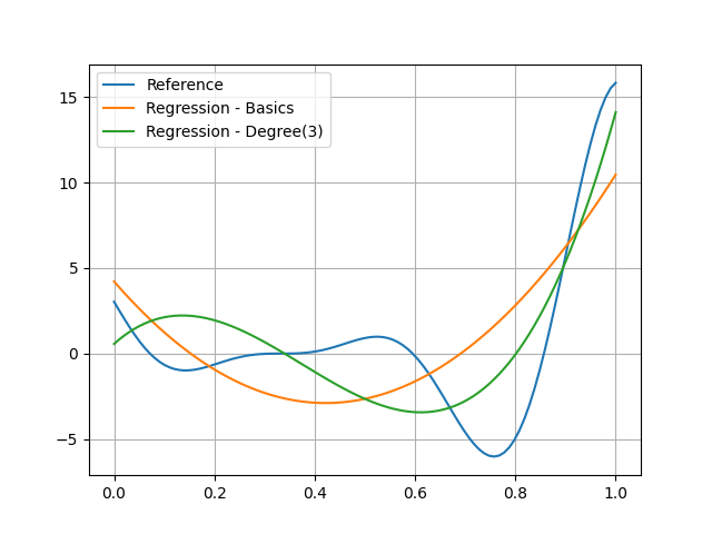
Degree

model = create_regression_model("PCERegressor", training_dataset, degree=3)
model.learn()

WARNING - 16:21:48: Remove input data transformation because PCERegressor does not support transformers.

and see that this model seems to be better:

predicted_output_data_ = model.predict(input_data).ravel()
plt.plot(input_data.ravel(), reference_output_data, label="Reference")
plt.plot(input_data.ravel(), predicted_output_data, label="Regression - Basics")
plt.plot(input_data.ravel(), predicted_output_data_, label="Regression - Degree(3)")
plt.grid()
plt.legend()
plt.show()