Sobol’ analysis

from __future__ import annotations

import pprint

from gemseo.algos.parameter_space import ParameterSpace
from gemseo.api import create_discipline
from gemseo.uncertainty.sensitivity.sobol.analysis import SobolAnalysis
from matplotlib import pyplot as plt
from numpy import pi

In this example, we consider a function from \([-\pi,\pi]^3\) to \(\mathbb{R}^3\):

\[(y_1,y_2)=\left(f(x_1,x_2,x_3),f(x_2,x_1,x_3)\right)\]

where \(f(a,b,c)=\sin(a)+7\sin(b)^2+0.1*c^4\sin(a)\) is the Ishigami function:

expressions = {
    "y1": "sin(x1)+7*sin(x2)**2+0.1*x3**4*sin(x1)",
    "y2": "sin(x2)+7*sin(x1)**2+0.1*x3**4*sin(x2)",
}
discipline = create_discipline(
    "AnalyticDiscipline", expressions=expressions, name="Ishigami2"
)

Then, we consider the case where the deterministic variables \(x_1\), \(x_2\) and \(x_3\) are replaced by the uncertain variables \(X_1\), \(X_2\) and \(X_3\). The latter are independent and identically distributed according to the uniform distribution between \(-\pi\) and \(\pi\):

uncertain_space = ParameterSpace()
for variable_name in ["x1", "x2", "x3"]:
    uncertain_space.add_random_variable(
        variable_name, "OTUniformDistribution", minimum=-pi, maximum=pi
    )

From that, we would like to carry out a sensitivity analysis with the random outputs \(Y_1=f(X_1,X_2,X_3)\) and \(Y_2=f(X_2,X_1,X_3)\). For that, we can compute the sensitivity indices from a SobolAnalysis:

sobol_analysis = SobolAnalysis([discipline], uncertain_space, 100)
sobol_analysis.main_method = "total"
sobol_analysis.compute_indices()

{'first': {'y2': [{'x1': array([0.75387699]), 'x2': array([0.26516667]), 'x3': array([0.35758815])}], 'y1': [{'x1': array([0.19426511]), 'x2': array([0.21211854]), 'x3': array([0.01782884])}]}, 'total': {'y2': [{'x1': array([0.36991381]), 'x2': array([0.60974968]), 'x3': array([0.34776012])}], 'y1': [{'x1': array([0.87052721]), 'x2': array([0.37726189]), 'x3': array([0.29945874])}]}}

The resulting indices are the first-order and total Sobol’ indices:

pprint.pprint(sobol_analysis.indices)

{'first': {'y1': [{'x1': array([0.19426511]),
                   'x2': array([0.21211854]),
                   'x3': array([0.01782884])}],
           'y2': [{'x1': array([0.75387699]),
                   'x2': array([0.26516667]),
                   'x3': array([0.35758815])}]},
 'total': {'y1': [{'x1': array([0.87052721]),
                   'x2': array([0.37726189]),
                   'x3': array([0.29945874])}],
           'y2': [{'x1': array([0.36991381]),
                   'x2': array([0.60974968]),
                   'x3': array([0.34776012])}]}}

They can also be accessed separately:

pprint.pprint(sobol_analysis.first_order_indices)
pprint.pprint(sobol_analysis.total_order_indices)

{'y1': [{'x1': array([0.19426511]),
         'x2': array([0.21211854]),
         'x3': array([0.01782884])}],
 'y2': [{'x1': array([0.75387699]),
         'x2': array([0.26516667]),
         'x3': array([0.35758815])}]}
{'y1': [{'x1': array([0.87052721]),
         'x2': array([0.37726189]),
         'x3': array([0.29945874])}],
 'y2': [{'x1': array([0.36991381]),
         'x2': array([0.60974968]),
         'x3': array([0.34776012])}]}

One can also obtain their confidence intervals:

pprint.pprint(sobol_analysis.get_intervals())
pprint.pprint(sobol_analysis.get_intervals(first_order=False))

{'y1': [{'x1': array([-0.03400625,  0.54199216]),
         'x2': array([-0.00512583,  0.66154825]),
         'x3': array([-0.40647314,  0.44110609])}],
 'y2': [{'x1': array([0.10944697, 1.99005049]),
         'x2': array([-0.31379805,  0.99720365]),
         'x3': array([-0.43222646,  1.8321417 ])}]}
{'y1': [{'x1': array([0.50048303, 1.91420643]),
         'x2': array([-0.35083774,  1.67786025]),
         'x3': array([-0.19380841,  1.59540502])}],
 'y2': [{'x1': array([-0.63775393,  3.12446122]),
         'x2': array([-0.01837286,  2.23112503]),
         'x3': array([-0.21486175,  1.97989239])}]}

The main indices are the total Sobol’ indices (SobolAnalysis.main_method can also be set to “first” to use the first-order indices as main indices):

pprint.pprint(sobol_analysis.main_indices)

{'y1': [{'x1': array([0.87052721]),
         'x2': array([0.37726189]),
         'x3': array([0.29945874])}],
 'y2': [{'x1': array([0.36991381]),
         'x2': array([0.60974968]),
         'x3': array([0.34776012])}]}

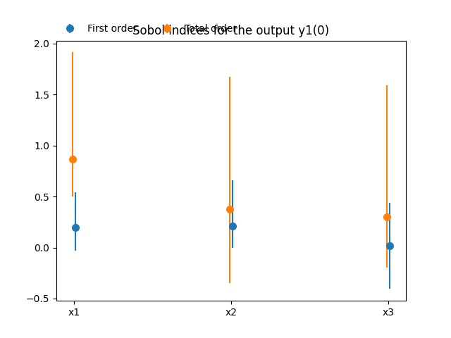
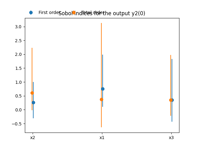
These main indices are used to sort the input parameters by decreasing order of influence. We can observe that this ranking is not the same for both outputs:

print(sobol_analysis.sort_parameters("y1"))
print(sobol_analysis.sort_parameters("y2"))

['x1', 'x2', 'x3']
['x2', 'x1', 'x3']

Lastly, we can use the method SobolAnalysis.plot() to visualize both first-order and total Sobol’ indices:

sobol_analysis.plot("y1", save=False, show=False)
sobol_analysis.plot("y2", save=False, show=False)
# Workaround for HTML rendering, instead of ``show=True``
plt.show()

• 
•