analysis module
Class for the estimation of Morris indices.
OAT technique
The purpose of the One-At-a-Time (OAT) methodology is to quantify the elementary effect
associated with a small variation \(dX_i\) of \(X_i\) with
The elementary effects \(df_1,\ldots,df_d\) are computed sequentially from an initial point
From these elementary effects, we can compare their absolute values \(|df_1|,\ldots,|df_d|\) and sort \(X_1,\ldots,X_d\) accordingly.
Morris technique
Then, the purpose of the Morris’ methodology is to repeat the OAT method from different initial points \(X^{(1)},\ldots,X^{(r)}\) and compare the parameters in terms of mean
and standard deviation
where \(\mu_i = \frac{1}{r}\sum_{j=1}^rdf_i^{(j)}\).
This methodology relies on the MorrisAnalysis class.
- class gemseo.uncertainty.sensitivity.morris.analysis.MorrisAnalysis(disciplines, parameter_space, n_samples, output_names=None, algo=None, algo_options=None, n_replicates=5, step=0.05, formulation='MDF', **formulation_options)[source]
Bases:
SensitivityAnalysisSensitivity analysis based on the Morris’ indices.
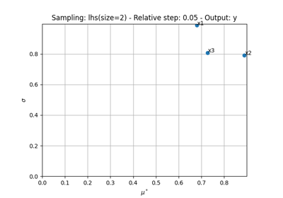
MorrisAnalysis.indicescontains both \(\mu^*\), \(\mu\) and \(\sigma\) whileMorrisAnalysis.main_indicesrepresents \(\mu^*\). Lastly, theMorrisAnalysis.plot()method represents the parameters as a scatter plot where \(X_i\) has as coordinates \((\mu_i^*,\sigma_i)\). The bigger \(\mu_i^*\) is, the more significant \(X_i\) is. Concerning \(\sigma_i\), it highlights non-linear effects along \(X_i\) or cross-effects between \(X_i\) and other parameter(s).The user can specify the DOE algorithm name to select the initial points, as well as the number of replicates and the relative step for the input variations.
Examples
>>> from numpy import pi
>>> from gemseo.api import create_discipline, create_parameter_space
>>> from gemseo.uncertainty.sensitivity.morris.analysis import MorrisAnalysis
>>>
>>> expressions = {"y": "sin(x1)+7*sin(x2)**2+0.1*x3**4*sin(x1)"}
>>> discipline = create_discipline(
...     "AnalyticDiscipline", expressions=expressions
... )
>>>
>>> parameter_space = create_parameter_space()
>>> parameter_space.add_random_variable(
...     "x1", "OTUniformDistribution", minimum=-pi, maximum=pi
... )
>>> parameter_space.add_random_variable(
...     "x2", "OTUniformDistribution", minimum=-pi, maximum=pi
... )
>>> parameter_space.add_random_variable(
...     "x3", "OTUniformDistribution", minimum=-pi, maximum=pi
... )
>>>
>>> analysis = MorrisAnalysis([discipline], parameter_space, n_samples=None)
>>> indices = analysis.compute_indices()
- Parameters:
disciplines (Collection[MDODiscipline]) – The discipline or disciplines to use for the analysis.
parameter_space (ParameterSpace) – A parameter space.
n_samples (int | None) – A number of samples. If
None, the number of samples is computed by the algorithm.output_names (Iterable[str] | None) – The disciplines’ outputs to be considered for the analysis. If
None, use all the outputs.algo (str | None) – The name of the DOE algorithm. If
None, use theSensitivityAnalysis.DEFAULT_DRIVER.algo_options (Mapping[str, DOELibraryOptionType] | None) – The options of the DOE algorithm.
n_replicates (int) –
The number of times the OAT method is repeated. Used only if
n_samplesis None. Otherwise, this number is the greater integer \(r\) such that \(r(d+1)\leq\)n_samplesand \(r(d+1)\) is the number of samples actually carried out.By default it is set to 5.
step (float) –
The finite difference step of the OAT method.
By default it is set to 0.05.
formulation (str) –
The name of the
MDOFormulationto sample the disciplines.By default it is set to “MDF”.
**formulation_options (Any) – The options of the
MDOFormulation.
- Raises:
ValueError – If at least one input dimension is not equal to 1.
- compute_indices(outputs=None, normalize=False)[source]
Compute the sensitivity indices.
- Parameters:
- Returns:
The sensitivity indices.
With the following structure:
{
    "method_name": {
        "output_name": [
            {
                "input_name": data_array,
            }
        ]
    }
}
- Return type:
- export_to_dataset()
Convert
SensitivityAnalysis.indicesinto aDataset.- Returns:
The sensitivity indices.
- Return type:
- static load(file_path)
Load a sensitivity analysis from the disk.
- Parameters:
file_path (str | Path) – The path to the file.
- Returns:
The sensitivity analysis.
- Return type:
- plot(output, inputs=None, title=None, save=True, show=False, file_path=None, directory_path=None, file_name=None, file_format=None, offset=1, lower_mu=None, lower_sigma=None)[source]
Plot the Morris indices for each input variable.
For \(i\in\{1,\ldots,d\}\), plot \(\mu_i^*\) in function of \(\sigma_i\).
- Parameters:
output (str | tuple[str, int]) – The output for which to display sensitivity indices, either a name or a tuple of the form (name, component). If name, its first component is considered.
inputs (Iterable[str] | None) – The inputs to display. If None, display all.
title (str | None) – The title of the plot. If None, no title.
save (bool) –
If True, save the figure.
By default it is set to True.
show (bool) –
If True, show the figure.
By default it is set to False.
file_path (str | Path | None) – A file path. Either a complete file path, a directory name or a file name. If None, use a default file name and a default directory. The file extension is inferred from filepath extension, if any.
directory_path (str | Path | None) – The description is missing.
file_name (str | None) – The description is missing.
file_format (str | None) – A file format, e.g. ‘png’, ‘pdf’, ‘svg’, … Used when
file_pathdoes not have any extension. If None, use a default file extension.offset (float) –
The offset to display the inputs names, expressed as a percentage applied to both x-range and y-range.
By default it is set to 1.
lower_mu (float | None) – The lower bound for \(\mu\). If None, use a default value.
lower_sigma (float | None) – The lower bound for \(\sigma\). If None, use a default value.
- Return type:
None
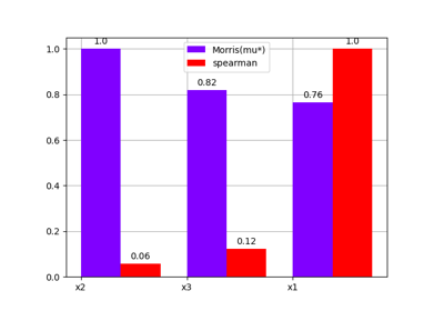
- plot_bar(outputs, inputs=None, standardize=False, title=None, save=True, show=False, file_path=None, directory_path=None, file_name=None, file_format=None, **options)
Plot the sensitivity indices on a bar chart.
This method may consider one or more outputs, as well as all inputs (default behavior) or a subset.
- Parameters:
outputs (OutputsType) – The outputs for which to display sensitivity indices, either a name, a list of names, a (name, component) tuple, a list of such tuples or a list mixing such tuples and names. When a name is specified, all its components are considered. If None, use the default outputs.
inputs (Iterable[str] | None) – The inputs to display. If None, display all.
standardize (bool) –
If True, standardize the indices between 0 and 1 for each output.
By default it is set to False.
title (str | None) – The title of the plot. If None, no title.
save (bool) –
If True, save the figure.
By default it is set to True.
show (bool) –
If True, show the figure.
By default it is set to False.
file_path (str | Path | None) – The path of the file to save the figures. If the extension is missing, use
file_extension. If None, create a file path fromdirectory_path,file_nameandfile_extension.directory_path (str | Path | None) – The path of the directory to save the figures. If None, use the current working directory.
file_name (str | None) – The name of the file to save the figures. If None, use a default one generated by the post-processing.
file_format (str | None) – A file extension, e.g. ‘png’, ‘pdf’, ‘svg’, … If None, use a default file extension.
options (int) –
- Returns:
A bar chart representing the sensitivity indices.
- Return type:
- plot_comparison(indices, output, inputs=None, title=None, use_bar_plot=True, save=True, show=False, file_path=None, directory_path=None, file_name=None, file_format=None, **options)
Plot a comparison between the current sensitivity indices and other ones.
This method allows to use either a bar chart (default option) or a radar one.
- Parameters:
indices (list[SensitivityAnalysis]) – The sensitivity indices.
output (str | tuple[str, int]) – The output for which to display sensitivity indices, either a name or a tuple of the form (name, component). If name, its first component is considered.
inputs (Iterable[str] | None) – The inputs to display. If None, display all.
title (str | None) – The title of the plot. If None, no title.
use_bar_plot (bool) –
The type of graph. If True, use a bar plot. Otherwise, use a radar chart.
By default it is set to True.
save (bool) –
If True, save the figure.
By default it is set to True.
show (bool) –
If True, show the figure.
By default it is set to False.
file_path (str | Path | None) – The path of the file to save the figures. If None, create a file path from
directory_path,file_nameandfile_format.directory_path (str | Path | None) – The path of the directory to save the figures. If None, use the current working directory.
file_name (str | None) – The name of the file to save the figures. If None, use a default one generated by the post-processing.
file_format (str | None) – A file format, e.g. ‘png’, ‘pdf’, ‘svg’, … If None, use a default file extension.
**options (bool) – The options passed to the underlying
DatasetPlot.
- Returns:
A graph comparing sensitivity indices.
- Return type:
- plot_field(output, mesh=None, inputs=None, standardize=False, title=None, save=True, show=False, file_path=None, directory_path=None, file_name=None, file_format=None, properties=None)
Plot the sensitivity indices related to a 1D or 2D functional output.
The output is considered as a 1D or 2D functional variable, according to the shape of the mesh on which it is represented.
- Parameters:
output (str | tuple[str, int]) – The output for which to display sensitivity indices, either a name or a tuple of the form (name, component) where (name, component) is used to sort the inputs. If it is a name, its first component is considered.
mesh (ndarray | None) – The mesh on which the p-length output is represented. Either a p-length array for a 1D functional output or a (p, 2) array for a 2D one. If None, assume a 1D functional output.
inputs (Iterable[str] | None) – The inputs to display. If None, display all inputs.
standardize (bool) –
If True, standardize the indices between 0 and 1 for each output.
By default it is set to False.
title (str | None) – The title of the plot. If None, no title is displayed.
save (bool) –
If True, save the figure.
By default it is set to True.
show (bool) –
If True, show the figure.
By default it is set to False.
file_path (str | Path | None) – The path of the file to save the figures. If None, create a file path from
directory_path,file_nameandfile_extension.directory_path (str | Path | None) – The path of the directory to save the figures. If None, use the current working directory.
file_name (str | None) – The name of the file to save the figures. If None, use a default one generated by the post-processing.
file_format (str | None) – A file extension, e.g. ‘png’, ‘pdf’, ‘svg’, … If None, use a default file extension.
properties (Mapping[str, DatasetPlotPropertyType]) – The general properties of a
DatasetPlot.
- Returns:
A bar plot representing the sensitivity indices.
- Raises:
NotImplementedError – If the dimension of the mesh is greater than 2.
- Return type:
- plot_radar(outputs, inputs=None, standardize=False, title=None, save=True, show=False, file_path=None, directory_path=None, file_name=None, file_format=None, min_radius=None, max_radius=None, **options)
Plot the sensitivity indices on a radar chart.
This method may consider one or more outputs, as well as all inputs (default behavior) or a subset.
For visualization purposes, it is also possible to change the minimum and maximum radius values.
- Parameters:
outputs (OutputsType) – The outputs for which to display sensitivity indices, either a name, a list of names, a (name, component) tuple, a list of such tuples or a list mixing such tuples and names. When a name is specified, all its components are considered. If None, use the default outputs.
inputs (Iterable[str] | None) – The inputs to display. If None, display all.
standardize (bool) –
If True, standardize the indices between 0 and 1 for each output.
By default it is set to False.
title (str | None) – The title of the plot. If None, no title.
save (bool) –
If True, save the figure.
By default it is set to True.
show (bool) –
If True, show the figure.
By default it is set to False.
file_path (str | Path | None) – The path of the file to save the figures. If the extension is missing, use
file_extension. If None, create a file path fromdirectory_path,file_nameandfile_extension.directory_path (str | Path | None) – The path of the directory to save the figures. If None, use the current working directory.
file_name (str | None) – The name of the file to save the figures. If None, use a default one generated by the post-processing.
file_format (str | None) – A file extension, e.g. ‘png’, ‘pdf’, ‘svg’, … If None, use a default file extension.
min_radius (float | None) – The minimal radial value. If None, from data.
max_radius (float | None) – The maximal radial value. If None, from data.
options (bool) –
- Returns:
A radar chart representing the sensitivity indices.
- Return type:
- save(file_path)
Save the current sensitivity analysis on the disk.
- Parameters:
file_path (str | Path) – The path to the file.
- Return type:
None
- sort_parameters(output)
Return the parameters sorted in descending order.
- Parameters:
output (str | tuple[str, int]) – Either a tuple as
(output_name, output_component)or an output name; in the second case, use the first output component.- Returns:
The input parameters sorted by decreasing order of sensitivity; in case of a multivariate input, aggregate the sensitivity indices associated to the different input components by adding them up typically.
- Return type:
- static standardize_indices(indices)
Standardize the sensitivity indices for each output component.
Each index is replaced by its absolute value divided by the largest index. Thus, the standardized indices belong to the interval \([0,1]\).
- DEFAULT_DRIVER = 'lhs'
- property indices: dict[str, Dict[str, List[Dict[str, numpy.ndarray]]]]
The sensitivity indices.
With the following structure:
{
    "method_name": {
        "output_name": [
            {
                "input_name": data_array,
            }
        ]
    }
}
- property main_indices: Dict[str, List[Dict[str, ndarray]]]
The main sensitivity indices.
With the following structure:
{
    "output_name": [
        {
            "input_name": data_array,
        }
    ]
}
- max: dict[str, dict[str, ndarray]]
The maximum effect with the following structure:
{
    "output_name": [
        {
            "input_name": data_array,
        }
    ]
}
- min: dict[str, dict[str, ndarray]]
The minimum effect with the following structure:
{
    "output_name": [
        {
            "input_name": data_array,
        }
    ]
}
- mu_: dict[str, dict[str, ndarray]]
The mean effects with the following structure:
{
    "output_name": [
        {
            "input_name": data_array,
        }
    ]
}
- mu_star: dict[str, dict[str, ndarray]]
The mean absolute effects with the following structure:
{
    "output_name": [
        {
            "input_name": data_array,
        }
    ]
}