Morris analysis

from __future__ import annotations

import pprint

from gemseo.uncertainty.sensitivity.morris.analysis import MorrisAnalysis
from gemseo.uncertainty.use_cases.ishigami.ishigami_discipline import IshigamiDiscipline
from gemseo.uncertainty.use_cases.ishigami.ishigami_space import IshigamiSpace

In this example, we consider the Ishigami function [IH90]

\[f(x_1,x_2,x_3)=\sin(x_1)+7\sin(x_2)^2+0.1x_3^4\sin(x_1)\]

implemented as an MDODiscipline by the IshigamiDiscipline. It is commonly used with the independent random variables \(X_1\), \(X_2\) and \(X_3\) uniformly distributed between \(-\pi\) and \(\pi\) and defined in the IshigamiSpace.

discipline = IshigamiDiscipline()
uncertain_space = IshigamiSpace()

Then, we run sensitivity analysis of type MorrisAnalysis:

sensitivity_analysis = MorrisAnalysis([discipline], uncertain_space, 10)
sensitivity_analysis.compute_indices()

{'mu': {'y': [{'x1': array([-0.36000398]), 'x2': array([0.77781853]), 'x3': array([-0.70990541])}]}, 'mu_star': {'y': [{'x1': array([0.67947346]), 'x2': array([0.88906579]), 'x3': array([0.72694219])}]}, 'sigma': {'y': [{'x1': array([0.98724949]), 'x2': array([0.79064599]), 'x3': array([0.8074493])}]}, 'relative_sigma': {'y': [{'x1': array([1.45296254]), 'x2': array([0.88929976]), 'x3': array([1.11074761])}]}, 'min': {'y': [{'x1': array([0.0338188]), 'x2': array([0.11821721]), 'x3': array([8.72820113e-05])}]}, 'max': {'y': [{'x1': array([2.2360336]), 'x2': array([1.83987522]), 'x3': array([2.12052546])}]}}

The resulting indices are the empirical means and the standard deviations of the absolute output variations due to input changes.

pprint.pprint(sensitivity_analysis.indices)

{'max': {'y': [{'x1': array([2.2360336]),
                'x2': array([1.83987522]),
                'x3': array([2.12052546])}]},
 'min': {'y': [{'x1': array([0.0338188]),
                'x2': array([0.11821721]),
                'x3': array([8.72820113e-05])}]},
 'mu': {'y': [{'x1': array([-0.36000398]),
               'x2': array([0.77781853]),
               'x3': array([-0.70990541])}]},
 'mu_star': {'y': [{'x1': array([0.67947346]),
                    'x2': array([0.88906579]),
                    'x3': array([0.72694219])}]},
 'relative_sigma': {'y': [{'x1': array([1.45296254]),
                           'x2': array([0.88929976]),
                           'x3': array([1.11074761])}]},
 'sigma': {'y': [{'x1': array([0.98724949]),
                  'x2': array([0.79064599]),
                  'x3': array([0.8074493])}]}}

The main indices corresponds to these empirical means (this main method can be changed with MorrisAnalysis.main_method):

pprint.pprint(sensitivity_analysis.main_indices)

{'y': [{'x1': array([0.67947346]),
        'x2': array([0.88906579]),
        'x3': array([0.72694219])}]}

and can be interpreted with respect to the empirical bounds of the outputs:

pprint.pprint(sensitivity_analysis.outputs_bounds)

{'y': [array([-1.42959705]), array([14.89344259])]}

We can also sort the input parameters by decreasing order of influence:

print(sensitivity_analysis.sort_parameters("y"))

['x2', 'x3', 'x1']

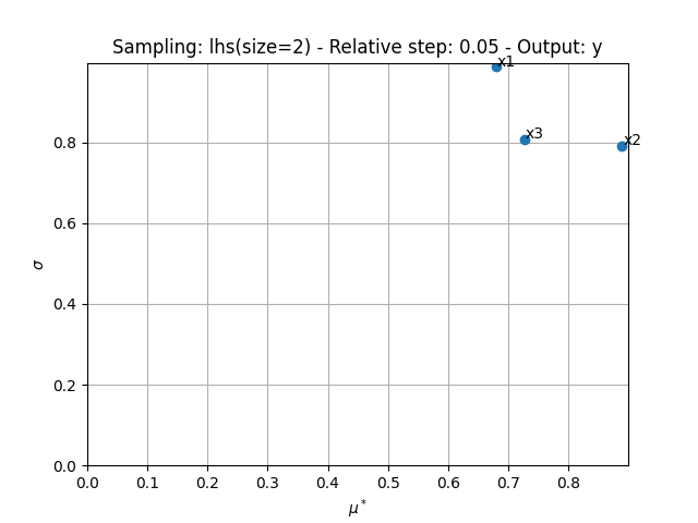
Lastly, we can use the method MorrisAnalysis.plot() to visualize the different series of indices:

sensitivity_analysis.plot("y", save=False, show=True, lower_mu=0, lower_sigma=0)