gemseo / uncertainty / sensitivity / sobol

analysis module¶

Class for the estimation of Sobol’ indices.

Let us consider the model \(Y=f(X_1,\ldots,X_d)\) where:

\(X_1,\ldots,X_d\) are independent random variables,
\(E\left[f(X_1,\ldots,X_d)^2\right]<\infty\).

Then, the following decomposition is unique:

\[Y=f_0 + \sum_{i=1}^df_i(X_i) + \sum_{i,j=1\atop i\neq j}^d f_{i,j}(X_i,X_j) + \sum_{i,j,k=1\atop i\neq j\neq k}^d f_{i,j,k}(X_i,X_j,X_k) + \ldots + f_{1,\ldots,d}(X_1,\ldots,X_d)\]

where:

\(f_0=E[Y]\),
\(f_i(X_i)=E[Y|X_i]-f_0\),
\(f_{i,j}(X_i,X_j)=E[Y|X_i,X_j]-f_i(X_i)-f_j(X_j)-f_0\)
and so on.

Then, the shift to variance leads to:

\[V[Y]=\sum_{i=1}^dV\left[f_i(X_i)\right] + \sum_{i,j=1\atop j\neq i}^d V\left[f_{i,j}(X_i,X_j)\right] + \ldots + V\left[f_{1,\ldots,d}(X_1,\ldots,X_d)\right]\]

and the Sobol’ indices are obtained by dividing by the variance and sum up to 1:

\[1=\sum_{i=1}^dS_i + \sum_{i,j=1\atop j\neq i}^d S_{i,j} + \sum_{i,j,k=1\atop i\neq j\neq k}^d S_{i,j,k} + \ldots + S_{1,\ldots,d}\]

A Sobol’ index represents the share of output variance explained by a parameter or a group of parameters. For the parameter \(X_i\),

\(S_i\) is the first-order Sobol’ index measuring the individual effect of \(X_i\),
\(S_{i,j}\) is the second-order Sobol’ index measuring the joint effect between \(X_i\) and \(X_j\),
\(S_{i,j,k}\) is the third-order Sobol’ index measuring the joint effect between \(X_i\), \(X_j\) and \(X_k\),
and so on.

In practice, we only consider the first-order Sobol’ index:

\[S_i=\frac{V[E[Y|X_i]]}{V[Y]}\]

and the total-order Sobol’ index:

\[S_i^T=\sum_{u\subset\{1,\ldots,d\}\atop u \ni i}S_u\]

The latter represents the sum of the individual effect of \(X_i\) and the joint effects between \(X_i\) and any parameter or group of parameters.

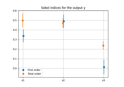
This methodology relies on the SobolAnalysis class. Precisely, SobolAnalysis.indices contains both SobolAnalysis.first_order_indices and SobolAnalysis.total_order_indices while SobolAnalysis.main_indices represents total-order Sobol’ indices. Lastly, the SobolAnalysis.plot() method represents the estimations of both first-order and total-order Sobol’ indices along with their confidence intervals whose default level is 95%.

The user can select the algorithm to estimate the Sobol’ indices. The computation relies on OpenTURNS capabilities.

class gemseo.uncertainty.sensitivity.sobol.analysis.SobolAnalysis(disciplines, parameter_space, n_samples, output_names=None, algo=None, algo_options=None, formulation='MDF', compute_second_order=True, use_asymptotic_distributions=True, **formulation_options)[source]¶

Bases: SensitivityAnalysis

Sensitivity analysis based on the Sobol’ indices.

Examples

>>> from numpy import pi
>>> from gemseo.api import create_discipline, create_parameter_space
>>> from gemseo.uncertainty.sensitivity.sobol.analysis import SobolAnalysis
>>>
>>> expressions = {"y": "sin(x1)+7*sin(x2)**2+0.1*x3**4*sin(x1)"}
>>> discipline = create_discipline(
...     "AnalyticDiscipline", expressions=expressions
... )
>>>
>>> parameter_space = create_parameter_space()
>>> parameter_space.add_random_variable(
...     "x1", "OTUniformDistribution", minimum=-pi, maximum=pi
... )
>>> parameter_space.add_random_variable(
...     "x2", "OTUniformDistribution", minimum=-pi, maximum=pi
... )
>>> parameter_space.add_random_variable(
...     "x3", "OTUniformDistribution", minimum=-pi, maximum=pi
... )
>>>
>>> analysis = SobolAnalysis([discipline], parameter_space, n_samples=10000)
>>> indices = analysis.compute_indices()

Parameters:

disciplines (Collection[MDODiscipline]) – The discipline or disciplines to use for the analysis.
parameter_space (ParameterSpace) – A parameter space.
n_samples (int) – A number of samples. If None, the number of samples is computed by the algorithm.
output_names (Iterable[str] | None) – The disciplines’ outputs to be considered for the analysis. If None, use all the outputs.
algo (str | None) – The name of the DOE algorithm. If None, use the SensitivityAnalysis.DEFAULT_DRIVER.
algo_options (Mapping[str, DOELibraryOptionType] | None) – The options of the DOE algorithm.
formulation (str) –
The name of the MDOFormulation to sample the disciplines.

By default it is set to “MDF”.
compute_second_order (bool) –
Whether to compute the second-order indices.

By default it is set to True.
use_asymptotic_distributions (bool) –
Whether to estimate the confidence intervals of the first- and total-order Sobol’ indices with the asymptotic distributions; otherwise, use bootstrap.

By default it is set to True.
**formulation_options (Any) – The options of the MDOFormulation.

Notes

The estimators of Sobol’ indices rely on the same DOE algorithm. This algorithm starts with two independent input datasets composed of \(N\) independent samples and this number \(N\) is the usual sampling size for Sobol’ analysis. When compute_second_order=False or when the input dimension \(d\) is equal to 2, \(N=\frac{n_\text{samples}}{2+d}\). Otherwise, \(N=\frac{n_\text{samples}}{2+2d}\). The larger \(N\), the more accurate the estimators of Sobol’ indices are. Therefore, for a small budget n_samples, the user can choose to set compute_second_order to False to ensure a better estimation of the first- and second-order indices.

class Algorithm(value)[source]¶

Bases: BaseEnum

The algorithms to estimate the Sobol’ indices.

Jansen(*args, **kwargs) = <class 'openturns.simulation.JansenSensitivityAlgorithm'>¶

Martinez(*args, **kwargs) = <class 'openturns.simulation.MartinezSensitivityAlgorithm'>¶

MauntzKucherenko(*args, **kwargs) = <class 'openturns.simulation.MauntzKucherenkoSensitivityAlgorithm'>¶

Saltelli(*args, **kwargs) = <class 'openturns.simulation.SaltelliSensitivityAlgorithm'>¶

class Method(value)[source]¶

Bases: BaseEnum

The names of the sensitivity methods.

first = 'Sobol(first)'¶

total = 'Sobol(total)'¶

compute_indices(outputs=None, algo=Algorithm.Saltelli, confidence_level=0.95)[source]¶

Compute the sensitivity indices.

Parameters:

outputs (Sequence[str] | None) – The outputs for which to display sensitivity indices. If None, use the default outputs, that are all the discipline outputs.
algo (Algorithm | str) –
The name of the algorithm to estimate the Sobol’ indices.

By default it is set to Saltelli.
confidence_level (float) –
The level of the confidence intervals.

By default it is set to 0.95.

Returns:

The sensitivity indices.

With the following structure:

{
    "method_name": {
        "output_name": [
            {
                "input_name": data_array,
            }
        ]
    }
}

Return type:

dict[str, IndicesType]

export_to_dataset()¶

Convert SensitivityAnalysis.indices into a Dataset.

Returns:: The sensitivity indices.
Return type:: Dataset

get_intervals(first_order=True)[source]¶

Get the confidence intervals for the Sobol’ indices.

Warning

You must first call compute_indices().

Parameters:

first_order (bool) –

If True, compute the intervals for the first-order indices. Otherwise, for the total-order indices.

By default it is set to True.

Returns:

The confidence intervals for the Sobol’ indices.

With the following structure:

{
    "output_name": [
        {
            "input_name": data_array,
        }
    ]
}

Return type:

Dict[str, List[Dict[str, ndarray]]]

static load(file_path)¶

Load a sensitivity analysis from the disk.

Parameters:: file_path (str | Path) – The path to the file.
Returns:: The sensitivity analysis.
Return type:: SensitivityAnalysis

plot(output, inputs=None, title=None, save=True, show=False, file_path=None, directory_path=None, file_name=None, file_format=None, sort=True, sort_by_total=True)[source]¶

Plot the first- and total-order Sobol’ indices.

For \(i\in\{1,\ldots,d\}\), plot \(S_i^{1}\) and \(S_T^{1}\) with their confidence intervals.

Parameters:

output (str | tuple[str, int]) – The output for which to display sensitivity indices, either a name or a tuple of the form (name, component). If name, its first component is considered.
inputs (Iterable[str] | None) – The inputs to display. If None, display all.
title (str | None) – The title of the plot. If None, no title.
save (bool) –
If True, save the figure.

By default it is set to True.
show (bool) –
If True, show the figure.

By default it is set to False.
file_path (str | Path | None) – A file path. Either a complete file path, a directory name or a file name. If None, use a default file name and a default directory. The file extension is inferred from filepath extension, if any.
directory_path (str | Path | None) – The description is missing.
file_name (str | None) – The description is missing.
file_format (str | None) – A file format, e.g. ‘png’, ‘pdf’, ‘svg’, … Used when file_path does not have any extension. If None, use a default file extension.
sort (bool) –
The sorting option. If True, sort variables before display.

By default it is set to True.
sort_by_total (bool) –
The type of sorting. If True, sort variables according to total-order Sobol’ indices. Otherwise, use first-order Sobol’ indices.

By default it is set to True.

plot_bar(outputs, inputs=None, standardize=False, title=None, save=True, show=False, file_path=None, directory_path=None, file_name=None, file_format=None, **options)¶

Plot the sensitivity indices on a bar chart.

This method may consider one or more outputs, as well as all inputs (default behavior) or a subset.

Parameters:

outputs (OutputsType) – The outputs for which to display sensitivity indices, either a name, a list of names, a (name, component) tuple, a list of such tuples or a list mixing such tuples and names. When a name is specified, all its components are considered. If None, use the default outputs.
inputs (Iterable[str] | None) – The inputs to display. If None, display all.
standardize (bool) –
If True, standardize the indices between 0 and 1 for each output.

By default it is set to False.
title (str | None) – The title of the plot. If None, no title.
save (bool) –
If True, save the figure.

By default it is set to True.
show (bool) –
If True, show the figure.

By default it is set to False.
file_path (str | Path | None) – The path of the file to save the figures. If the extension is missing, use file_extension. If None, create a file path from directory_path, file_name and file_extension.
directory_path (str | Path | None) – The path of the directory to save the figures. If None, use the current working directory.
file_name (str | None) – The name of the file to save the figures. If None, use a default one generated by the post-processing.
file_format (str | None) – A file extension, e.g. ‘png’, ‘pdf’, ‘svg’, … If None, use a default file extension.
options (int) –

Returns:

A bar chart representing the sensitivity indices.

Return type:

BarPlot

plot_comparison(indices, output, inputs=None, title=None, use_bar_plot=True, save=True, show=False, file_path=None, directory_path=None, file_name=None, file_format=None, **options)¶

Plot a comparison between the current sensitivity indices and other ones.

This method allows to use either a bar chart (default option) or a radar one.

Parameters:

indices (list[SensitivityAnalysis]) – The sensitivity indices.
output (str | tuple[str, int]) – The output for which to display sensitivity indices, either a name or a tuple of the form (name, component). If name, its first component is considered.
inputs (Iterable[str] | None) – The inputs to display. If None, display all.
title (str | None) – The title of the plot. If None, no title.
use_bar_plot (bool) –
The type of graph. If True, use a bar plot. Otherwise, use a radar chart.

By default it is set to True.
save (bool) –
If True, save the figure.

By default it is set to True.
show (bool) –
If True, show the figure.

By default it is set to False.
file_path (str | Path | None) – The path of the file to save the figures. If None, create a file path from directory_path, file_name and file_format.
directory_path (str | Path | None) – The path of the directory to save the figures. If None, use the current working directory.
file_name (str | None) – The name of the file to save the figures. If None, use a default one generated by the post-processing.
file_format (str | None) – A file format, e.g. ‘png’, ‘pdf’, ‘svg’, … If None, use a default file extension.
**options (bool) – The options passed to the underlying DatasetPlot.

Returns:

A graph comparing sensitivity indices.

Return type:

BarPlot | RadarChart

plot_field(output, mesh=None, inputs=None, standardize=False, title=None, save=True, show=False, file_path=None, directory_path=None, file_name=None, file_format=None, properties=None)¶

Plot the sensitivity indices related to a 1D or 2D functional output.

The output is considered as a 1D or 2D functional variable, according to the shape of the mesh on which it is represented.

Parameters:

output (str | tuple[str, int]) – The output for which to display sensitivity indices, either a name or a tuple of the form (name, component) where (name, component) is used to sort the inputs. If it is a name, its first component is considered.
mesh (ndarray | None) – The mesh on which the p-length output is represented. Either a p-length array for a 1D functional output or a (p, 2) array for a 2D one. If None, assume a 1D functional output.
inputs (Iterable[str] | None) – The inputs to display. If None, display all inputs.
standardize (bool) –
If True, standardize the indices between 0 and 1 for each output.

By default it is set to False.
title (str | None) – The title of the plot. If None, no title is displayed.
save (bool) –
If True, save the figure.

By default it is set to True.
show (bool) –
If True, show the figure.

By default it is set to False.
file_path (str | Path | None) – The path of the file to save the figures. If None, create a file path from directory_path, file_name and file_extension.
directory_path (str | Path | None) – The path of the directory to save the figures. If None, use the current working directory.
file_name (str | None) – The name of the file to save the figures. If None, use a default one generated by the post-processing.
file_format (str | None) – A file extension, e.g. ‘png’, ‘pdf’, ‘svg’, … If None, use a default file extension.
properties (Mapping[str, DatasetPlotPropertyType]) – The general properties of a DatasetPlot.

Returns:

A bar plot representing the sensitivity indices.

Raises:

NotImplementedError – If the dimension of the mesh is greater than 2.

Return type:

Curves | Surfaces

plot_radar(outputs, inputs=None, standardize=False, title=None, save=True, show=False, file_path=None, directory_path=None, file_name=None, file_format=None, min_radius=None, max_radius=None, **options)¶

Plot the sensitivity indices on a radar chart.

This method may consider one or more outputs, as well as all inputs (default behavior) or a subset.

For visualization purposes, it is also possible to change the minimum and maximum radius values.

Parameters:

outputs (OutputsType) – The outputs for which to display sensitivity indices, either a name, a list of names, a (name, component) tuple, a list of such tuples or a list mixing such tuples and names. When a name is specified, all its components are considered. If None, use the default outputs.
inputs (Iterable[str] | None) – The inputs to display. If None, display all.
standardize (bool) –
If True, standardize the indices between 0 and 1 for each output.

By default it is set to False.
title (str | None) – The title of the plot. If None, no title.
save (bool) –
If True, save the figure.

By default it is set to True.
show (bool) –
If True, show the figure.

By default it is set to False.
file_path (str | Path | None) – The path of the file to save the figures. If the extension is missing, use file_extension. If None, create a file path from directory_path, file_name and file_extension.
directory_path (str | Path | None) – The path of the directory to save the figures. If None, use the current working directory.
file_name (str | None) – The name of the file to save the figures. If None, use a default one generated by the post-processing.
file_format (str | None) – A file extension, e.g. ‘png’, ‘pdf’, ‘svg’, … If None, use a default file extension.
min_radius (float | None) – The minimal radial value. If None, from data.
max_radius (float | None) – The maximal radial value. If None, from data.
options (bool) –

Returns:

A radar chart representing the sensitivity indices.

Return type:

RadarChart

save(file_path)¶

Save the current sensitivity analysis on the disk.

Parameters:: file_path (str | Path) – The path to the file.
Return type:: None

sort_parameters(output)¶

Return the parameters sorted in descending order.

Parameters:: output (str | tuple[str, int]) – Either a tuple as (output_name, output_component) or an output name; in the second case, use the first output component.
Returns:: The input parameters sorted by decreasing order of sensitivity; in case of a multivariate input, aggregate the sensitivity indices associated to the different input components by adding them up typically.
Return type:: list[str]

static standardize_indices(indices)¶

Standardize the sensitivity indices for each output component.

Each index is replaced by its absolute value divided by the largest index. Thus, the standardized indices belong to the interval \([0,1]\).

Parameters:: indices (Dict[str, List[Dict[str, ndarray]]]) – The indices to be standardized.
Returns:: The standardized indices.
Return type:: Dict[str, List[Dict[str, ndarray]]]

AVAILABLE_ALGOS: ClassVar[list[str]] = ['Jansen', 'Martinez', 'MauntzKucherenko', 'Saltelli']¶: The names of the available algorithms to estimate the Sobol’ indices.

DEFAULT_DRIVER: ClassVar[str] = 'OT_SOBOL_INDICES'¶

dataset: Dataset¶: The dataset containing the discipline evaluations.

default_output: list[str]¶: The default outputs of interest.

property first_order_indices: Dict[str, List[Dict[str, ndarray]]]¶

The first-order Sobol’ indices.

With the following structure:

{
    "output_name": [
        {
            "input_name": data_array,
        }
    ]
}

property indices: dict[str, Dict[str, List[Dict[str, numpy.ndarray]]]]¶

The sensitivity indices.

With the following structure:

{
    "method_name": {
        "output_name": [
            {
                "input_name": data_array,
            }
        ]
    }
}

property inputs_names: list[str]¶: The names of the inputs.

property main_indices: Dict[str, List[Dict[str, ndarray]]]¶

The main sensitivity indices.

With the following structure:

{
    "output_name": [
        {
            "input_name": data_array,
        }
    ]
}

property main_method: str¶: The name of the main method.

property second_order_indices: Dict[str, List[Dict[str, ndarray]]]¶

The second-order Sobol’ indices.

With the following structure:

{
    "output_name": [
        {
            "input_name": data_array,
        }
    ]
}

property total_order_indices: Dict[str, List[Dict[str, ndarray]]]¶

The total-order Sobol’ indices.

With the following structure:

{
    "output_name": [
        {
            "input_name": data_array,
        }
    ]
}

Examples using SobolAnalysis¶

Sobol’ analysis

Sobol' analysis