Optimization History View

In this example, we illustrate the use of the OptHistoryView plot on the Sobieski’s SSBJ problem.

from __future__ import annotations

from gemseo import configure_logger
from gemseo import create_discipline
from gemseo import create_scenario
from gemseo.problems.sobieski.core.design_space import SobieskiDesignSpace

Import

The first step is to import some high-level functions and a method to get the design space.

configure_logger()

<RootLogger root (INFO)>

Description

The OptHistoryView post-processing creates a series of plots:

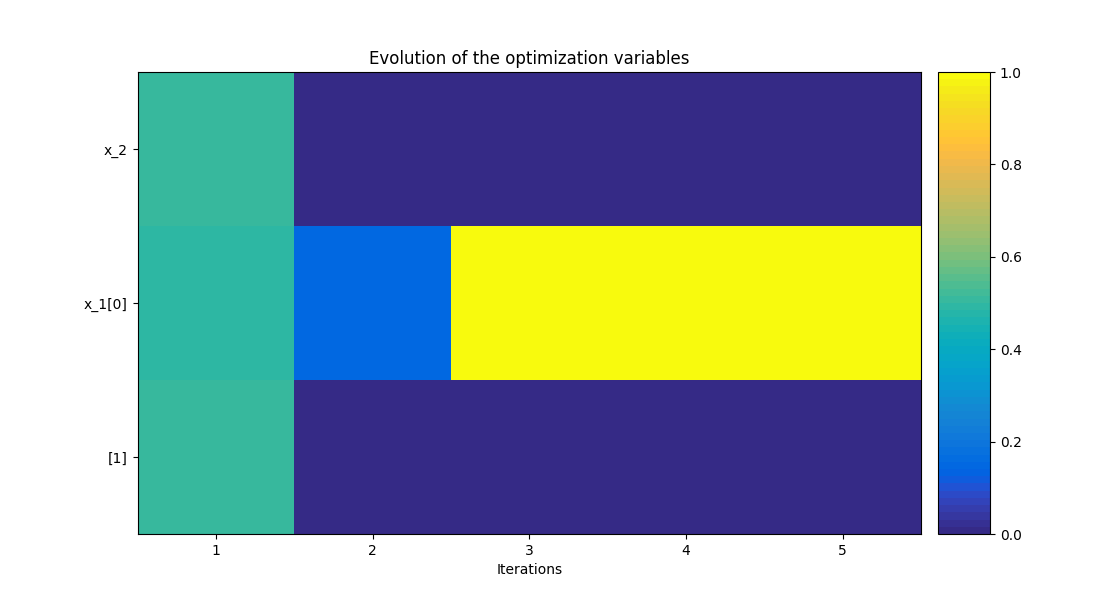
• The design variables history - This graph shows the normalized values of the design variables, the \(y\) axis is the index of the inputs in the vector; and the \(x\) axis represents the iterations.

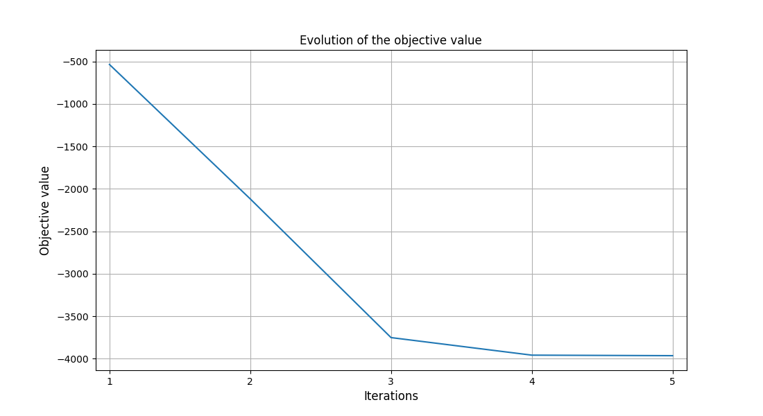
• The objective function history - It shows the evolution of the objective value during the optimization.

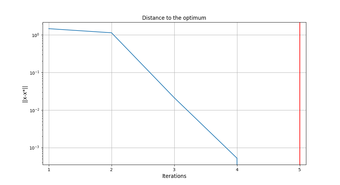
• The distance to the best design variables - Plots the vector \(log( ||x-x^*|| )\) in log scale.

• The history of the Hessian approximation of the objective - Plots an approximation of the second order derivatives of the objective function \(\frac{\partial^2 f(x)}{\partial x^2}\), which is a measure of the sensitivity of the function with respect to the design variables, and of the anisotropy of the problem (differences of curvatures in the design space).

• The inequality constraint history - Portrays the evolution of the values of the constraints. The inequality constraints must be non-positive, that is why the plot must be green or white for satisfied constraints (white = active, red = violated). For an IDF formulation, an additional plot is created to track the equality constraint history.

Create disciplines

At this point we instantiate the disciplines of Sobieski’s SSBJ problem: Propulsion, Aerodynamics, Structure and Mission

disciplines = create_discipline([
    "SobieskiPropulsion",
    "SobieskiAerodynamics",
    "SobieskiStructure",
    "SobieskiMission",
])

Create design space

We also create the SobieskiDesignSpace.

design_space = SobieskiDesignSpace()

Create and execute scenario

The next step is to build an MDO scenario in order to maximize the range, encoded ‘y_4’, with respect to the design parameters, while satisfying the inequality constraints ‘g_1’, ‘g_2’ and ‘g_3’. We can use the MDF formulation, the SLSQP optimization algorithm and a maximum number of iterations equal to 100.

scenario = create_scenario(
    disciplines,
    "MDF",
    "y_4",
    design_space,
    maximize_objective=True,
)
scenario.set_differentiation_method()
for constraint in ["g_1", "g_2", "g_3"]:
    scenario.add_constraint(constraint, constraint_type="ineq")
scenario.execute({"algo": "SLSQP", "max_iter": 100})

    INFO - 13:57:12:
    INFO - 13:57:12: *** Start MDOScenario execution ***
    INFO - 13:57:12: MDOScenario
    INFO - 13:57:12:    Disciplines: SobieskiAerodynamics SobieskiMission SobieskiPropulsion SobieskiStructure
    INFO - 13:57:12:    MDO formulation: MDF
    INFO - 13:57:12: Optimization problem:
    INFO - 13:57:12:    minimize -y_4(x_shared, x_1, x_2, x_3)
    INFO - 13:57:12:    with respect to x_1, x_2, x_3, x_shared
    INFO - 13:57:12:    subject to constraints:
    INFO - 13:57:12:       g_1(x_shared, x_1, x_2, x_3) <= 0.0
    INFO - 13:57:12:       g_2(x_shared, x_1, x_2, x_3) <= 0.0
    INFO - 13:57:12:       g_3(x_shared, x_1, x_2, x_3) <= 0.0
    INFO - 13:57:12:    over the design space:
    INFO - 13:57:12:       +-------------+-------------+-------+-------------+-------+
    INFO - 13:57:12:       | Name        | Lower bound | Value | Upper bound | Type  |
    INFO - 13:57:12:       +-------------+-------------+-------+-------------+-------+
    INFO - 13:57:12:       | x_shared[0] |     0.01    |  0.05 |     0.09    | float |
    INFO - 13:57:12:       | x_shared[1] |    30000    | 45000 |    60000    | float |
    INFO - 13:57:12:       | x_shared[2] |     1.4     |  1.6  |     1.8     | float |
    INFO - 13:57:12:       | x_shared[3] |     2.5     |  5.5  |     8.5     | float |
    INFO - 13:57:12:       | x_shared[4] |      40     |   55  |      70     | float |
    INFO - 13:57:12:       | x_shared[5] |     500     |  1000 |     1500    | float |
    INFO - 13:57:12:       | x_1[0]      |     0.1     |  0.25 |     0.4     | float |
    INFO - 13:57:12:       | x_1[1]      |     0.75    |   1   |     1.25    | float |
    INFO - 13:57:12:       | x_2         |     0.75    |   1   |     1.25    | float |
    INFO - 13:57:12:       | x_3         |     0.1     |  0.5  |      1      | float |
    INFO - 13:57:12:       +-------------+-------------+-------+-------------+-------+
    INFO - 13:57:12: Solving optimization problem with algorithm SLSQP:
    INFO - 13:57:12:      1%|          | 1/100 [00:00<00:09, 10.44 it/sec, obj=-536]
    INFO - 13:57:12:      2%|▏         | 2/100 [00:00<00:13,  7.19 it/sec, obj=-2.12e+3]
 WARNING - 13:57:12: MDAJacobi has reached its maximum number of iterations but the normed residual 1.7130677857005655e-05 is still above the tolerance 1e-06.
    INFO - 13:57:12:      3%|▎         | 3/100 [00:00<00:15,  6.10 it/sec, obj=-3.75e+3]
    INFO - 13:57:12:      4%|▍         | 4/100 [00:00<00:16,  5.86 it/sec, obj=-3.96e+3]
    INFO - 13:57:12:      5%|▌         | 5/100 [00:00<00:16,  5.71 it/sec, obj=-3.96e+3]
    INFO - 13:57:13: Optimization result:
    INFO - 13:57:13:    Optimizer info:
    INFO - 13:57:13:       Status: 8
    INFO - 13:57:13:       Message: Positive directional derivative for linesearch
    INFO - 13:57:13:       Number of calls to the objective function by the optimizer: 6
    INFO - 13:57:13:    Solution:
    INFO - 13:57:13:       The solution is feasible.
    INFO - 13:57:13:       Objective: -3963.408265187933
    INFO - 13:57:13:       Standardized constraints:
    INFO - 13:57:13:          g_1 = [-0.01806104 -0.03334642 -0.04424946 -0.0518346  -0.05732607 -0.13720865
    INFO - 13:57:13:  -0.10279135]
    INFO - 13:57:13:          g_2 = 3.333278582928756e-06
    INFO - 13:57:13:          g_3 = [-7.67181773e-01 -2.32818227e-01  8.30379541e-07 -1.83255000e-01]
    INFO - 13:57:13:       Design space:
    INFO - 13:57:13:          +-------------+-------------+---------------------+-------------+-------+
    INFO - 13:57:13:          | Name        | Lower bound |        Value        | Upper bound | Type  |
    INFO - 13:57:13:          +-------------+-------------+---------------------+-------------+-------+
    INFO - 13:57:13:          | x_shared[0] |     0.01    | 0.06000083331964572 |     0.09    | float |
    INFO - 13:57:13:          | x_shared[1] |    30000    |        60000        |    60000    | float |
    INFO - 13:57:13:          | x_shared[2] |     1.4     |         1.4         |     1.8     | float |
    INFO - 13:57:13:          | x_shared[3] |     2.5     |         2.5         |     8.5     | float |
    INFO - 13:57:13:          | x_shared[4] |      40     |          70         |      70     | float |
    INFO - 13:57:13:          | x_shared[5] |     500     |         1500        |     1500    | float |
    INFO - 13:57:13:          | x_1[0]      |     0.1     |         0.4         |     0.4     | float |
    INFO - 13:57:13:          | x_1[1]      |     0.75    |         0.75        |     1.25    | float |
    INFO - 13:57:13:          | x_2         |     0.75    |         0.75        |     1.25    | float |
    INFO - 13:57:13:          | x_3         |     0.1     |  0.1562448753887276 |      1      | float |
    INFO - 13:57:13:          +-------------+-------------+---------------------+-------------+-------+
    INFO - 13:57:13: *** End MDOScenario execution (time: 0:00:01.000171) ***

{'max_iter': 100, 'algo': 'SLSQP'}

Post-process scenario

Lastly, we post-process the scenario by means of the OptHistoryView plot which plots the history of optimization for both objective function, constraints, design parameters and distance to the optimum.

Tip

Each post-processing method requires different inputs and offers a variety of customization options. Use the high-level function get_post_processing_options_schema() to print a table with the options for any post-processing algorithm. Or refer to our dedicated page: Post-processing algorithms.

scenario.post_process(
    "OptHistoryView", save=False, show=True, variable_names=["x_2", "x_1"]
)

• 
• 
• 
• 
• 

<gemseo.post.opt_history_view.OptHistoryView object at 0x7f2d10bb8dc0>