
MDO formulations#
In this section we describe the MDO formulations features of GEMSEO.
Available formulations in GEMSEO#
To see which formulations are available in your GEMSEO version, you may have a look in the folder gemseo.formulations.
Another possibility is to use the API method gemseo.get_available_formulations() to list them:
from gemseo import get_available_formulations
print(get_available_formulations())
This prints the formulations names available in the current configuration.
['BiLevel', 'BiLevelBCD', 'DisciplinaryOpt', 'IDF', 'MDF']
- These implement the classical formulations:
Multi-Disciplinary Feasible (MDF);
Individual Discipline Feasible (IDF);
a simple disciplinary optimization formulation for a weakly coupled problem;
another bi-level formulation, denoted Bi-level Block Coordinate Descent (Bi-level BCD) formulation, from IRT Saint-Exupéry that enhances the previous one with a Block Coordinate Descent (BCD) algorithm.
In the following, general concepts about the formulations are given. The MDF and IDF text is integrally taken from the paper [VGM17].
To see how to setup practical test cases with such formulations, please see A from scratch example on the Sellar problem and Application: Sobieski's Super-Sonic Business Jet (MDO).
See also
For a review of MDO formulations, see [ML13].
We use the following notations:
\(N\) is the number of disciplines,
\(x=(x_1,x_2,\ldots,x_N)\) are the local design variables,
\(z\) are the shared design variables,
\(y=(y_1,y_2,\ldots,y_N)=\Psi(x, z)\) are the coupling variables,
\(f\) is the objective,
\(g\) are the constraints.
MDF#
MDF is an architecture that guarantees an equilibrium between all disciplines at each iterate \((x, z)\) of the optimization process. Consequently, should the optimization process be prematurely interrupted, the best known solution has a physical meaning. MDF generates the smallest possible optimization problem, in which the coupling variables are removed from the set of optimization variables and the residuals removed from the set of constraints:
The coupling variables \(y(x, z)\) are computed at equilibrium via an MDA. It amounts to solving a system of (possibly nonlinear) equations using fixed-point methods (Gauss-Seidel, Jacobi) or root-finding methods (Newton-Raphson, quasi-Newton). A prerequisite for invoking is the existence of an equilibrium for any values of the design variables \((x, z)\) encountered during the optimization process.

A process based on the MDF formulation.#
Gradient-based optimization algorithms require the computation of the total derivatives of \(\phi(x, z, y(x, z))\), where \(\phi \in \{f, g\}\) and \(v \in \{x, z\}\).
For details on the MDAs and coupled derivatives, see Multi Disciplinary Analyses and Coupled derivatives and gradients computation.
An example of an MDO study using an MDF formulation can be found in the A from scratch example on the Sellar problem example.
Warning
Any Discipline that will be placed inside an MDF formulation with strong couplings must
define its default inputs. Otherwise, the execution will fail.
IDF#
IDF stands for individual discipline feasible. This MDO formulation expresses the MDO problem as
where \(y^t=(y_1^t,y_2^t,\ldots,y_N^t)\) are additional optimization variables, called targets or coupling targets, used as input coupling variables of the disciplines. The additional constraints \(y_i(x_i, z, y^t_{j \neq i}) - y_i^t = 0, \forall i \in \{1, \ldots, N\}\), called consistency constraints, ensure that the output coupling variables computed by the disciplines \(y\) coincide with the targets.
The use of coupling targets allows the disciplines to be run in a decoupled way while the use of consistency constraints guarantees a multidisciplinary feasible solution at convergence of the optimizer. Thus, the iterations are less costly than those of MDF, as they do not use an MDA algorithm, but IF does not allow early stopping with the guarantee of a multidisciplinary feasible solution, unlike MDF.
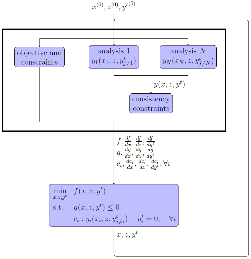
A process based on the IDF formulation.#
Note that the targets can include either all the couplings or the strong couplings only. If all couplings, then all disciplines are executed in parallel, and all couplings (weak and strong) are set as target variables in the design space. This maximizes the exploitation of the parallelism but leads to a larger design space, so usually more iterations by the optimizer.

The XDSM of the IDF formulation for the Sobieski's SSBJ problem, considering all the coupling targets.#
If the strong couplings only, then the coupling graph is analyzed and the disciplines are chained in sequence and in parallel to solve all weak couplings. In this case, the size of the optimization problem is reduced, so usually leads to less iterations. The best option depends on the number of strong vs weak couplings, the availability of gradients, the availability of CPUs versus the number of disciplines, so it is very context dependant.

The XDSM of the IDF formulation for the Sobieski's SSBJ problem, considering the strong coupling targets only.#
Bi-level#
Bi-level formulations are a family of MDO formulations that involve multiple optimization problems to be solved to obtain the solution of the MDO problem.
In many of them, and in particular in the formulations derived from BLISS, the separation of the optimization problems is made on the design variables. The design variables shared by multiple disciplines are put in a so-called system level optimization problem. In so-called disciplinary optimization problems, only the design variables that have a direct impact on one discipline are used. Then, the coupling variables may be solved by a Multi Disciplinary Analyses, as in formulations derived from MDF (BLISS, ASO or CSSO), or by using consistency constraints or a penalty function, like in IDF-like formulations (CO or ATC).
The next figure shows the decomposition of the Bi-level MDO formulation implemented in GEMSEO with two MDAs, the parallel sub-optimizations and a main optimization (system level) on the shared variables. It is an MDF-based approach, derived from the BLISS 98 formulation and variants from ONERA [BILD12]. This formulation was invented in the MDA-MDO project at IRT Saint-Exupéry [GGG+17], [GGA+19] and also used in the R-EVOL project [GAG+24].
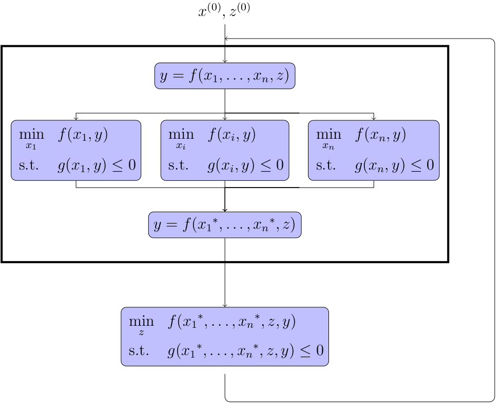
A process based on a Bi-level formulation.#
This block decomposition is motivated by several purposes. First, this separation aligns with the industrial needs of work repartition between domains, which matches the decomposition in terms of disciplines. It allows for greater flexibility in the use of specific approaches (algorithms) for solving disciplinary optimizations, also dealing with less design variables at the same time. Secondly, as the full coupled derivatives may not be available, the use of a gradient-based approach with all variables in the loop may not be affordable.
In the current Bi-level formulation, the objective function is minimized block by block, in parallel, with each block \(i\) minimizing its own variables \(x_i\) and handling its own constraints \(g_i\). Sometimes, if it is not straightforward to optimize the objective function \(f\) in the sub-problem \(i\), another function \(f_i\) can be considered as long as its decay is consistent with the decay (monotonic decrease) of the overall objective function \(f\). The decomposition is such that the sub-problems constraints \(g_i\) are assumed to depend on other block variables \(x_{\neq i}\) only through the couplings. These couplings are solved by two MDAs: one before the sub-optimizations in order to compute equilibrium values for each block, and the second one after the sub-optimizations in order to recompute the equilibrium for system level functions. The sub-optimization blocks do not exchange any information when they are solved in parallel, which means that the synchronization is ensured by the two MDAs and the system iterations which warm start each block with the previous optimal values of local variables. If the effect of one block variables \(x_i\) on another block \(j\) is too significant, it means that the optimal solution \(x^*\) is sensitive to the initial guess \(x\), and therefore that for same values of shared variables \(z\), different solutions \(x^*\) can be obtained. As a consequence, the synchronization mechanism may not be sufficient to solve accurately the lower problem and the system level algorithm may not converge to the right solution. In such a situation, an enhancement is proposed with the Bi-level Block Coordinate Descent (Bi-level BCD) which extends the range of problems that can be solved with Bi-level approaches.
An example of the Bi-level formulation implemented on the Sobieski SSBJ test case can be found in BiLevel-based MDO on the Sobieski SSBJ test case.
Warning
Any Discipline that will be placed inside a BiLevel
formulation with strong couplings must define its default inputs.
Otherwise, the execution will fail.
Bi-level Block Coordinate Descent (Bi-level BCD)#
The Bi-level BCD formulation adds more robustness and stability with respect to the previous Bi-level formulation, solving more accurately the inner sub-problem. The decomposition discussed in the previous Bi-level section remains the same and motivated by the same considerations. The next figure shows the process corresponding to the Bi-level BCD implemented in GEMSEO. This formulation was invented in the R-EVOL project at IRT Saint-Exupéry and more details can be found in [Dav24] and [DGR24].

A process based on a Bi-level BCD formulation.#
Here, it can be seen that the lower problem is solved by a Block Coordinate Descent method (BCD), also known as the Block Gauss-Seidel method (BGS), which means that each block, consisting of a disciplinary optimization, is sequentially optimized within an iterative loop until convergence. As a consequence, each block \(i\) is updated at every BCD iteration with \(x_{\neq i}^*\) until a fixed point \(x^*\) is found, regardless the initial guess \(x\), which drastically reduces the discrepancy of lower level solutions with respect to same values of shared variables.
In [DGR24], several variants are discussed, regarding the way how the couplings are solved:
when all the couplings are solved by running MDAs within each sub-optimization, the formulation is referred to as the Bi-level BCD-MDF;
when each sub-optimization no longer solves the whole coupling vector but only its own block of coupling variables, similarly to the design vector \(x_i\), the formulation is referred to as the Bi-level BCD-WK (stands for weak BCD). In this case, both the design variables and the coupling variables are exchanged through the BCD loop and updated at each sub-optimization. This approach can be considered either when running MDAs in each sub-optimization is too time consuming, or when it is simply not accessible due to tools limitation that do not give access to all coupling functions.
The Bi-level BCD process schematized in the above image corresponds to the Bi-level BCD-MDF version where all the couplings are solved within each block, which is explicitly denoted by the dependence of \(f\) and \(g_i\) to \(\Psi(x, z)\), meaning that the couplings are recomputed and not fixed during sub-optimization conversely to the previous Bi-level. While MDA 1 and 2 may not be theoretically necessary, in practice they allow to respectively compute more relevant initial coupling values for the BCD loop and objective function and constraints values for the system level optimizers when the BCD loop is not fully or not enough converged.
An example of the Bi-level BCD-MDF formulation implemented on the Sobieski SSBJ test case can be found in Bi-level BCD-based MDO on the Sobieski SSBJ test case.
XDSM visualization#
GEMSEO allows to visualize a given MDO scenario/formulation as an XDSM diagram (see [LM12]) in a web browser. The figure below shows an example of such visualization.
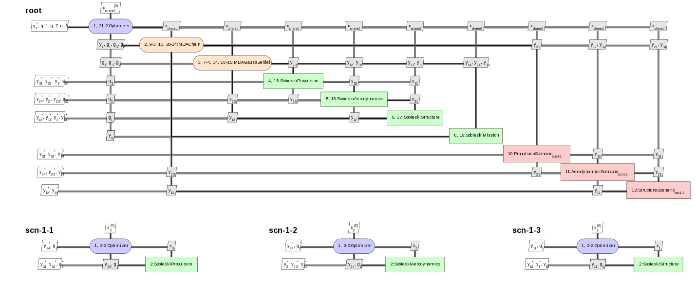
An XDSM visualization generated with GEMSEO.#
The rendering is handled by the visualization library XDSMjs.
GEMSEO provides a utility class XDSMizer to export the given MDO scenario as a suitable
input json file for this visualization library.
Features#
XDSM visualization shows:
dataflow between disciplines (connections between disciplines as list of variables)
optimization problem display (click on optimizer box)
workflow animation (top-left contol buttons trigger either automatic or step-by-step mode)
Those features are illustrated by the animated gif below.
GEMSEO XDSM visualization of the Sobiesky example solved with MDF formulation.#
Usage#
Then within your Python script, given your scenario object, you can generate the XDSM json file
with the following code:
scenario.xdsmize(show_html=True)
If save_html (default True), will generate a self contained HTML file, that can be automatically open using the option show_html=True.
If save_json is True, it will generate a XDSMjs input file XDSM visualization (legacy behavior).
If save_pdf=True (default False), a LaTex PDF is generated.
You should observe the XDSM diagram related to your MDO scenario.